| Type: | Package |
| Title: | Antarctic Spatial Data Manipulation |
| Version: | 4.2.1 |
| Date: | 2025-02-17 |
| Description: | Loads and creates spatial data, including layers and tools that are relevant to the activities of the Commission for the Conservation of Antarctic Marine Living Resources. Provides two categories of functions: load functions and create functions. Load functions are used to import existing spatial layers from the online CCAMLR GIS such as the ASD boundaries. Create functions are used to create layers from user data such as polygons and grids. |
| Depends: | R (≥ 4.0), sf |
| License: | GPL-3 |
| URL: | https://github.com/ccamlr/CCAMLRGIS#ccamlrgis-r-package |
| Encoding: | UTF-8 |
| LazyData: | true |
| Imports: | dplyr, terra, graphics, grDevices, magrittr, isoband, bezier, lwgeom |
| RoxygenNote: | 7.3.2 |
| Suggests: | knitr, rmarkdown, testthat |
| VignetteBuilder: | knitr |
| NeedsCompilation: | no |
| Packaged: | 2025-02-16 22:51:10 UTC; stephane |
| Author: | Stephane Thanassekos [aut, cre], Keith Reid [aut], Lucy Robinson [aut], Michael D. Sumner [ctb], Roger Bivand [ctb] |
| Maintainer: | Stephane Thanassekos <stephane.thanassekos@ccamlr.org> |
| Repository: | CRAN |
| Date/Publication: | 2025-02-17 00:10:24 UTC |
Loads and creates spatial data, including layers and tools that are relevant to CCAMLR activities. All operations use the Lambert azimuthal equal-area projection (via EPSG:6932).
Description
This package provides two broad categories of functions: load functions and create functions.
Load functions
Load functions are used to import CCAMLR geo-referenced layers and include:
Create functions
Create functions are used to create geo-referenced layers from user-generated data and include:
Vignette
To learn more about CCAMLRGIS, start with the GitHub ReadMe (see https://github.com/ccamlr/CCAMLRGIS#ccamlrgis-r-package). Some basemaps are given here https://github.com/ccamlr/CCAMLRGIS/blob/master/Basemaps/Basemaps.md
Author(s)
Maintainer: Stephane Thanassekos stephane.thanassekos@ccamlr.org
Authors:
Keith Reid
Lucy Robinson
Other contributors:
Michael D. Sumner [contributor]
Roger Bivand [contributor]
See Also
The CCAMLRGIS package relies on several other package which users may want to familiarize themselves with, namely sf (https://CRAN.R-project.org/package=sf) and terra (https://CRAN.R-project.org/package=terra).
CCAMLRGIS Projection
Description
The CCAMLRGIS package uses the Lambert azimuthal equal-area projection (see https://en.wikipedia.org/wiki/Lambert_azimuthal_equal-area_projection). Source: https://gis.ccamlr.org/. In order to align with recent developments within Geographic Information Software, this projection will be accessed via EPSG code 6932 (see https://epsg.org/crs_6932/WGS-84-NSIDC-EASE-Grid-2-0-South.html).
Usage
data(CCAMLRp)
Format
character string
Value
"+proj=laea +lat_0=-90 +lon_0=0 +x_0=0 +y_0=0 +datum=WGS84 +units=m +no_defs"
Clip Polygons to a simplified Antarctic coastline
Description
Clip Polygons to the Coast (removes polygon parts that fall on land) and computes the area of the resulting polygon. Uses an sf object as input which may be user-generated or created via buffered points (see create_Points), buffered lines (see create_Lines) or polygons (see create_Polys). N.B.: this function uses a simplified coastline. For more accurate results, load the high resolution coastline (see load_Coastline), and use sf::st_difference().
Usage
Clip2Coast(Input)
Arguments
Input |
sf polygon(s) to be clipped. |
Value
sf polygon carrying the same data as the Input.
See Also
Coast, create_Points, create_Lines, create_Polys,
create_PolyGrids.
Examples
MyPolys=create_Polys(PolyData,Densify=TRUE,Buffer=c(10,-15,120))
plot(st_geometry(MyPolys),col='red')
plot(st_geometry(Coast[Coast$ID=='All',]),add=TRUE)
MyPolysClipped=Clip2Coast(MyPolys)
plot(st_geometry(MyPolysClipped),col='blue',add=TRUE)
#View(MyPolysClipped)
Simplified and subsettable coastline
Description
Coastline polygons generated from load_Coastline and sub-sampled to only contain data that falls within the boundaries of the Convention Area. This spatial object may be subsetted to plot the coastline for selected ASDs or EEZs (see examples). Source: https://gis.ccamlr.org/
Usage
data(Coast)
Format
sf
See Also
Examples
#Complete coastline:
plot(st_geometry(Coast[Coast$ID=='All',]),col='grey')

#ASD 48.1 coastline:
plot(st_geometry(Coast[Coast$ID=='48.1',]),col='grey')
Bathymetry colors
Description
Set of standard colors to plot bathymetry, to be used in conjunction with Depth_cuts.
Usage
data(Depth_cols)
Format
character vector
See Also
Depth_cols2, add_col, add_Cscale, SmallBathy.
Examples
terra::plot(SmallBathy(),breaks=Depth_cuts,col=Depth_cols,axes=FALSE)
Bathymetry colors with Fishable Depth range
Description
Set of colors to plot bathymetry and highlight Fishable Depth range (600-1800), to be used in conjunction with Depth_cuts2.
Usage
data(Depth_cols2)
Format
character vector
See Also
Depth_cols, add_col, add_Cscale, SmallBathy.
Examples
terra::plot(SmallBathy(),breaks=Depth_cuts2,col=Depth_cols2,axes=FALSE,box=FALSE)
Bathymetry depth classes
Description
Set of depth classes to plot bathymetry, to be used in conjunction with Depth_cols.
Usage
data(Depth_cuts)
Format
numeric vector
See Also
Depth_cuts2, add_col, add_Cscale, SmallBathy.
Examples
terra::plot(SmallBathy(),breaks=Depth_cuts,col=Depth_cols,axes=FALSE,box=FALSE)
Bathymetry depth classes with Fishable Depth range
Description
Set of depth classes to plot bathymetry and highlight Fishable Depth range (600-1800), to be used in conjunction with Depth_cols2.
Usage
data(Depth_cuts2)
Format
numeric vector
See Also
Depth_cuts, add_col, add_Cscale, SmallBathy.
Examples
terra::plot(SmallBathy(),breaks=Depth_cuts2,col=Depth_cols2,axes=FALSE,box=FALSE)
Example dataset for create_PolyGrids
Description
To be used in conjunction with create_PolyGrids.
Usage
data(GridData)
Format
data.frame
See Also
Examples
#View(GridData)

MyGrid=create_PolyGrids(Input=GridData,dlon=2,dlat=1)
plot(st_geometry(MyGrid),col=MyGrid$Col_Catch_sum)
Polygon labels
Description
Labels for the layers obtained via 'load_' functions. Positions correspond to the centroids
of polygon parts. Can be used in conjunction with add_labels.
Usage
data(Labels)
Format
data.frame
See Also
add_labels, load_ASDs, load_SSRUs, load_RBs,
load_SSMUs, load_MAs, load_EEZs,
load_MPAs.
Examples
#View(Labels)

ASDs=load_ASDs()
plot(st_geometry(ASDs))
add_labels(mode='auto',layer='ASDs',fontsize=1,fonttype=2)
Example dataset for create_Lines
Description
To be used in conjunction with create_Lines.
Usage
data(LineData)
Format
data.frame
See Also
Examples
#View(LineData)

MyLines=create_Lines(LineData)
plot(st_geometry(MyLines),lwd=2,col=rainbow(5))
Example dataset for create_Pies
Description
To be used in conjunction with create_Pies. Count and catch of species per location.
Usage
data(PieData)
Format
data.frame
See Also
Examples
#View(PieData)

#Create pies
MyPies=create_Pies(Input=PieData,
                   NamesIn=c("Lat","Lon","Sp","N"),
                   Size=50
)
#Plot Pies
plot(st_geometry(MyPies),col=MyPies$col)
#Add Pies legend
add_PieLegend(Pies=MyPies,PosX=-0.1,PosY=-1.6,Boxexp=c(0.5,0.45,0.12,0.45),
              PieTitle="Species")
Example dataset for create_Pies
Description
To be used in conjunction with create_Pies. Count and catch of species per location.
Usage
data(PieData2)
Format
data.frame
See Also
Examples
#View(PieData2)

MyPies=create_Pies(Input=PieData2,
                  NamesIn=c("Lat","Lon","Sp","N"),
                  Size=5,
                  GridKm=250
)
#Plot Pies
plot(st_geometry(MyPies),col=MyPies$col)
#Add Pies legend
add_PieLegend(Pies=MyPies,PosX=-0.8,PosY=-0.3,Boxexp=c(0.5,0.45,0.12,0.45),
             PieTitle="Species")
Example dataset for create_Points
Description
To be used in conjunction with create_Points.
Usage
data(PointData)
Format
data.frame
See Also
Examples
#View(PointData)

MyPoints=create_Points(PointData)
plot(st_geometry(MyPoints))
text(MyPoints$x,MyPoints$y,MyPoints$name,adj=c(0.5,-0.5),xpd=TRUE)
plot(st_geometry(MyPoints[MyPoints$name=='four',]),bg='red',pch=21,cex=1.5,add=TRUE)
Example dataset for create_Polys
Description
To be used in conjunction with create_Polys.
Usage
data(PolyData)
Format
data.frame
See Also
Examples
#View(PolyData)

MyPolys=create_Polys(PolyData,Densify=TRUE)
plot(st_geometry(MyPolys),col='green')
text(MyPolys$Labx,MyPolys$Laby,MyPolys$ID)
plot(st_geometry(MyPolys[MyPolys$ID=='three',]),border='red',lwd=3,add=TRUE)
Rotate object
Description
Rotate a spatial object by setting the longitude that should point up.
Usage
Rotate_obj(Input, Lon0 = NULL)
Arguments
Input |
Spatial object of class |
Lon0 |
numeric, longitude that will point up in the resulting map. |
Value
Spatial object in your environment to only be used for plotting, not for analysis.
See Also
create_Points, create_Lines, create_Polys,
create_PolyGrids, create_Stations, create_Pies,
create_Arrow.
Examples
# For more examples, see:
# https://github.com/ccamlr/CCAMLRGIS#47-rotate_obj
# and:
# https://github.com/ccamlr/CCAMLRGIS/blob/master/Basemaps/Basemaps.md

RotB=Rotate_obj(SmallBathy(),Lon0=-180)
terra::plot(RotB,breaks=Depth_cuts,col=Depth_cols,axes=FALSE,box=FALSE,legend=FALSE)
add_RefGrid(bb=st_bbox(RotB),ResLat=10,ResLon=20,LabLon = -180,offset = 3)
Small bathymetry dataset
Description
Bathymetry dataset derived from the GEBCO 2024 (see https://www.gebco.net/) dataset.
Subsampled at a 10,000m resolution. Projected using the CCAMLR standard projection (CCAMLRp).
To highlight the Fishable Depth range, use Depth_cols2 and Depth_cuts2.
To be only used for large scale illustrative purposes. Please refer to load_Bathy
to get higher resolution data.
Usage
SmallBathy()
Format
raster
References
GEBCO Compilation Group (2024) GEBCO 2024 Grid (doi:10.5285/1c44ce99-0a0d-5f4f-e063-7086abc0ea0f)
See Also
load_Bathy, add_col, add_Cscale, Depth_cols,
Depth_cuts,
Depth_cols2, Depth_cuts2, get_depths, create_Stations.
Examples
terra::plot(SmallBathy(),breaks=Depth_cuts,col=Depth_cols,axes=FALSE,box=FALSE)
Add a color scale
Description
Adds a color scale to plots. Default behavior set for bathymetry. May also be used to
place a legend.
Usage
add_Cscale(
  pos = "1/1",
  title = "Depth (m)",
  width = 18,
  height = 70,
  cuts = Depth_cuts,
  cols = Depth_cols,
  minVal = NA,
  maxVal = NA,
  fontsize = 1,
  offset = 100,
  lwd = 1,
  Titlefontsize = 1.2 * fontsize,
  TitleVAdj = 0,
  BoxAdj = c(0, 0, 0, 0),
  BoxCol = "black",
  BoxBG = "white",
  Clwd = 0,
  Ccol = "black",
  Cwdth = 1,
  TckL = 1,
  Tcklwd = 1,
  Tdist = 1,
  mode = "Cscale"
)
Arguments
pos |
character, fraction indicating the vertical position of the color scale (which, by default, is on the
right side of plots). if |
title |
character, title of the color scale. |
width |
numeric, width of the color scale box, expressed in % of the width of the plotting region. |
height |
numeric, height of the color scale box, expressed in % of the height of the plotting region. |
cuts |
numeric, vector of color classes. May be generated via |
cols |
character, vector of color names. May be generated via |
minVal |
numeric, if desired, the color scale may be generated starting from the value |
maxVal |
numeric, if desired, the color scale may be generated up to the value |
fontsize |
numeric, size of the text in the color scale. |
offset |
numeric, controls the horizontal position of the color scale. |
lwd |
numeric, thickness of lines. |
Titlefontsize |
numeric, size of the title text. |
TitleVAdj |
numeric, vertical adjustment of the title. |
BoxAdj |
numeric vector of 4 values to adjust the sides of the box, given as |
BoxCol |
Color of the legend box frame. |
BoxBG |
Color of the legend box background. |
Clwd |
numeric, thickness of lines of cells. |
Ccol |
character, color of lines of cells, set to NA for no border. |
Cwdth |
numeric, positive factor to adjust the width of cells. |
TckL |
numeric, positive factor to adjust the length of tick lines. |
Tcklwd |
numeric, thickness of tick lines. |
Tdist |
numeric, horizontal adjustment of labels text. |
mode |
character, if 'Cscale', the default, the function builds a color scale. if 'Legend', the function
gives you the location of a |
See Also
load_Bathy, SmallBathy, Depth_cuts, Depth_cols,
Depth_cuts2, Depth_cols2, add_col, add_Legend,
R colors, legend.
Examples
# For more examples, see:
# https://github.com/ccamlr/CCAMLRGIS#5-adding-colors-legends-and-labels

library(terra)

#Example 1: Adding two color scales

plot(SmallBathy(),breaks=Depth_cuts,col=Depth_cols,legend=FALSE,axes=FALSE,box=FALSE)
add_Cscale(pos='1/2',height=45,maxVal=0,minVal=-4000,fontsize=0.8)
#Some gridded data
MyGrid=create_PolyGrids(GridData,dlon=2,dlat=1)
Gridcol=add_col(MyGrid$Catch_sum,cuts=10)
plot(st_geometry(MyGrid),col=Gridcol$varcol,add=TRUE)
#Add color scale using cuts and cols generated by add_col, note the use of 'round'
add_Cscale(pos='2/2',height=45,title='Catch (t)',
           cuts=round(Gridcol$cuts,1),cols=Gridcol$cols,fontsize=0.8)

#Example 2: Adding a color scale and a legend

#Create some point data
MyPoints=create_Points(PointData)

#Crop the bathymetry to match the extent of MyPoints

BathyCr=crop(SmallBathy(),extend(ext(MyPoints),100000))
plot(BathyCr,breaks=Depth_cuts,col=Depth_cols,legend=FALSE,axes=FALSE,mar=c(0,0,0,7))
add_Cscale(pos='1/2',height=45,maxVal=0,minVal=-4000,fontsize=0.8)

#Plot points with different symbols and colors (see ?points)
Psymbols=c(21,22,23,24)
Pcolors=c('red','green','blue','yellow')
plot(st_geometry(MyPoints[MyPoints$name=='one',]),pch=Psymbols[1],bg=Pcolors[1],add=TRUE)
plot(st_geometry(MyPoints[MyPoints$name=='two',]),pch=Psymbols[2],bg=Pcolors[2],add=TRUE)
plot(st_geometry(MyPoints[MyPoints$name=='three',]),pch=Psymbols[3],bg=Pcolors[3],add=TRUE)
plot(st_geometry(MyPoints[MyPoints$name=='four',]),pch=Psymbols[4],bg=Pcolors[4],add=TRUE)

#Add legend with position determined by add_Cscale
Loc=add_Cscale(pos='2/2',height=45,mode='Legend')
legend(Loc,legend=c('one','two','three','four'),title='Vessel',pch=Psymbols,
pt.bg=Pcolors,xpd=TRUE)
Add Legend
Description
Add a legend to you map. Give the bounding box of your plot and lists of parameters as inputs.
Usage
add_Legend(bb, LegOpt, Items)
Arguments
bb |
bounding box of your plot area. for example,
|
LegOpt |
list of general legend options. for example:
|
Items |
list, or list of lists containing options for each item to be displayed in the legend. for example:
|
Value
Legend added to current plot.
LegOpt options
Title: character, title of the legend, set to NULL for no title.
Subtitle: character, subtitle of the legend, set to NULL for no subtitle.
Pos: character, general position of the legend. One of "bottomright" (default), "bottom", "bottomleft", "left", "topleft", "top", "topright", "right" or "center".
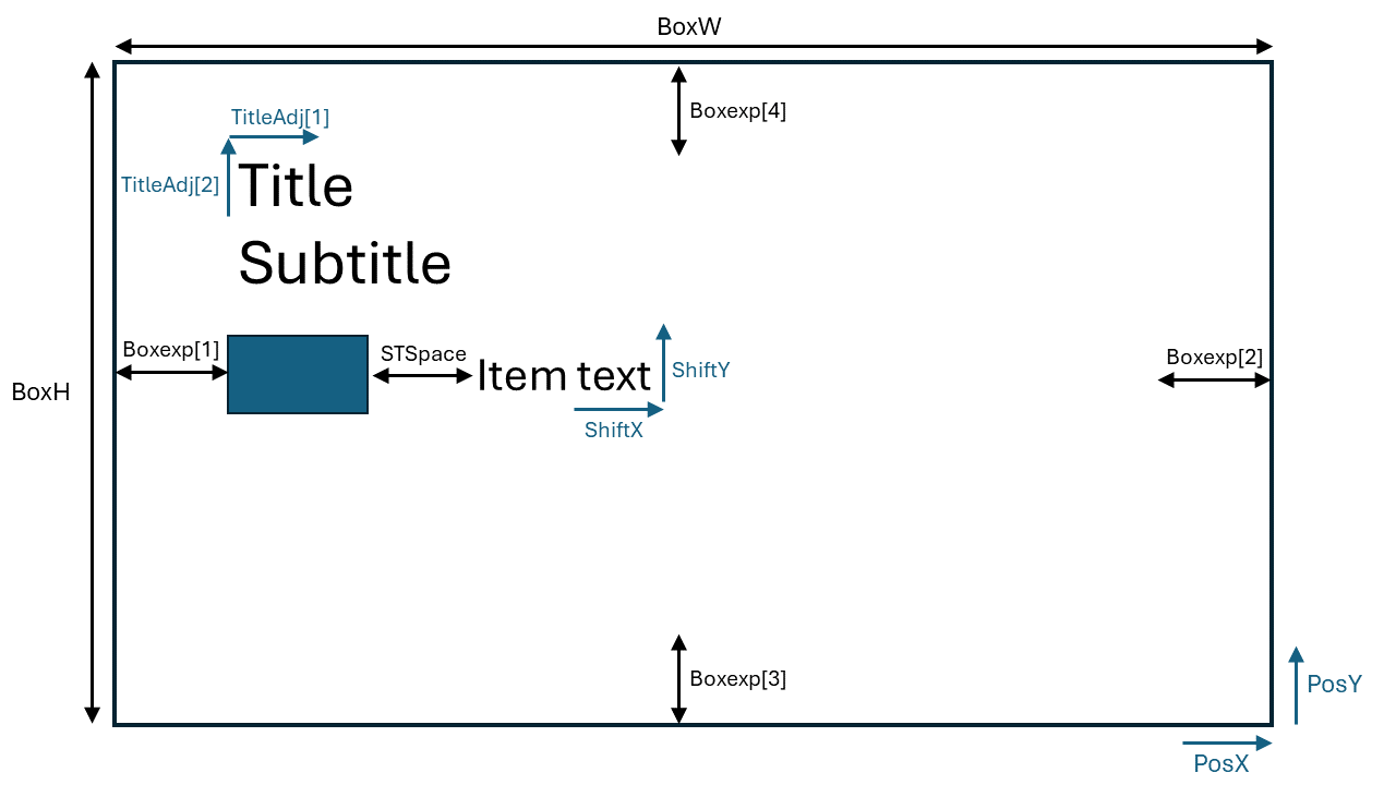
BoxW: numeric, legend box width (see figure below).
BoxH: numeric, legend box height (see figure below).
PosX: numeric, horizontal adjustment of legend (see figure below).
PosY: numeric, vertical adjustment of legend (see figure below).
Boxexp: numeric, vector of length 4 controlling the expansion of the legend box, given as c(xmin,xmax,ymin,ymax), see figure below.
Boxbd: character, color of the background of the legend box. set to NA for no background.
Boxcol: character, color of the border of the legend box. Set to NA for no box.
Boxlwd: numeric, line thickness of the legend box. Set Boxcol to NA for no box.
Titlefontsize: numeric, size of the legend title.
Subtitlefontsize: numeric, size of the legend subtitle.
TitleAdj: numeric vector of length 2, as c(x,y) to adjust title location (see figure below).
SubtitleAdj: numeric vector of length 2, as c(x,y) to adjust subtitle location.
Items options that are common to all items
Text: character, text of the item.
Shape: character, shape description, one of "rectangle", "circle", "ellipse", "line", "arrow" or "none". Using "none" will leave a blank space that can be filled by a user-defined shape.
ShpFill: character, fill color of shape, set to NA for no fill.
ShpBord: character, border color of shape, set to NA for no border.
ShpHash: logical (TRUE/FALSE) to add hashed lines to the shape (see create_Hashes).
Shplwd: numeric, line thickness of the shape's border, set ShpBord to NA for no border.
fontsize: numeric, size of the text.
STSpace: numeric, space between the Shape and its Text (see figure below).
ShiftX: numeric, shift Shape and Text left or right (see figure below).
ShiftY: numeric, shift Shape and Text up or down (see figure below).
Hashcol: character, color of hashes (if ShpHash is TRUE), see create_Hashes for details.
Hashangle: numeric, angle of hashes (if ShpHash is TRUE), see create_Hashes for details.
Hashspacing: numeric, spacing between hashes (if ShpHash is TRUE), see create_Hashes for details.
Hashwidth: numeric, width of hashes (if ShpHash is TRUE), see see create_Hashes for details.
Items options that are specific to the item's Shape
RectW: numeric, width of rectangle shape.
RectH: numeric, height of rectangle shape.
CircD: numeric, diameter of circle shape.
EllW: numeric, width of ellipse shape.
EllH: numeric, height of ellipse shape.
EllA: numeric, angle of ellipse shape.
LineTyp: numeric, type of line shape (0=blank, 1=solid, 2=dashed, 3=dotted, 4=dotdash, 5=longdash, 6=twodash).
LineL: numeric, length of the line shape.
ArrL: numeric, length of the arrow shape.
ArrPwidth: numeric, width of arrow's path. see create_Arrow for details.
ArrHlength: numeric, length of arrow's head. see create_Arrow for details.
ArrHwidth: numeric, width of arrow's head. see create_Arrow for details.
Arrdlength: numeric, length of dashes for dashed arrows. see create_Arrow for details.
Arrtype: character, arrow type either "normal" or "dashed". see create_Arrow for details.
Arrcol: character, color of the arrow. see create_Arrow for details.
Arrtrans: numeric, transparency of the arrow. see create_Arrow for details.
The figure below shows some of the options used to customize the legend box and its items. Blue arrows represent location options and black arrows represent sizing options:
See Also
create_Hashes, create_Arrow, create_Ellipse,
add_labels, add_Cscale, add_PieLegend.
Examples
# For more examples, see:
# https://github.com/ccamlr/CCAMLRGIS#53-adding-legends

# Set general options:

LegOpt=list(
Title= "Title",
Subtitle="(Subtitle)",
Pos = "bottomright",
BoxW= 80,
BoxH= 170,
Boxexp = c(5,-2,-4,-4),
Titlefontsize = 2
)


#Create separate items, each with their own options:


Rectangle1=list(
  Text="Rectangle 1",
  Shape="rectangle",
  ShpFill="cyan",
  ShpBord="blue",
  Shplwd=2,
  fontsize=1.2,
  STSpace=3,
  RectW=10,
  RectH=7
)

Rectangle2=list(
  Text="Rectangle 2",
  Shape="rectangle",
  ShpFill="red",
  ShpBord="orange",
  ShpHash=TRUE,
  Shplwd=2,
  fontsize=1.2,
  STSpace=3,
  RectW=10,
  RectH=7,
  Hashcol="white",
  Hashangle=45,
  Hashspacing=1,
  Hashwidth=1
)

Circle1=list(
  Text="Circle 1",
  Shape="circle",
  ShpFill="grey",
  ShpBord="yellow",
  Shplwd=2,
  fontsize=1.2,
  STSpace=3,
  CircD=10
)

Circle2=list(
  Text="Circle 2",
  Shape="circle",
  ShpFill="white",
  ShpBord="red",
  ShpHash=TRUE,
  Shplwd=2,
  fontsize=1.2,
  STSpace=3,
  CircD=10,
  Hashcol="black",
  Hashangle=0,
  Hashspacing=2,
  Hashwidth=2
)

Ellipse1=list(
  Text="Ellipse 1",
  Shape="ellipse",
  ShpFill="white",
  ShpBord="darkblue",
  Shplwd=2,
  fontsize=1.2,
  STSpace=3,
  EllW=10,
  EllH=6,
  EllA=35
)

Ellipse2=list(
  Text="Ellipse 2",
  Shape="ellipse",
  ShpFill="red",
  ShpBord="green",
  ShpHash=TRUE,
  Shplwd=2,
  fontsize=1.2,
  STSpace=3,
  EllW=10,
  EllH=7,
  EllA=0,
  Hashcol="black",
  Hashangle=-45,
  Hashspacing=1.5,
  Hashwidth=1.5
)

Line1=list(
  Text="Line 1",
  Shape="line",
  ShpFill="black",
  Shplwd=5,
  fontsize=1.2,
  STSpace=3,
  LineL=10
)

Line2=list(
  Text="Line 2",
  Shape="line",
  Shplwd=5,
  ShpFill="green",
  Shplwd=5,
  fontsize=1.2,
  STSpace=3,
  LineTyp=6,
  LineL=10
)

Arrow1=list(
  Text="Arrow 1",
  Shape="arrow",
  ShpBord="green",
  Shplwd=1,
  ArrL=10,
  ArrPwidth=5,
  ArrHlength=15,
  ArrHwidth=10,
  Arrcol="orange",
  fontsize=1.2,
  STSpace=3
)

Arrow2=list(
  Text="Arrow 2",
  Shape="arrow",
  ShpBord=NA,
  ArrL=10,
  ArrPwidth=5,
  ArrHlength=15,
  ArrHwidth=10,
  Arrdlength=0,
  Arrtype="dashed",
  Arrcol=c("red","green","blue"),
  fontsize=1.2,
  STSpace=3
)

Arrow3=list(
  Text="Arrow 3",
  Shape="arrow",
  ShpBord=NA,
  ArrL=10,
  ArrPwidth=5,
  ArrHlength=15,
  ArrHwidth=10,
  Arrdlength=5,
  Arrtype="dashed",
  Arrcol="darkgreen",
  fontsize=1.2,
  STSpace=3
)

Arrow4=list(
  Text="Arrow 4",
  Shape="arrow",
  ShpBord="black",
  Shplwd=0.1,
  ArrL=10,
  ArrPwidth=5,
  ArrHlength=15,
  ArrHwidth=10,
  Arrcol="pink",
  ShpHash=TRUE,
  Hashcol="blue",
  Hashangle=-45,
  Hashspacing=1,
  Hashwidth=1,
  fontsize=1.2,
  STSpace=3
)

None=list(
  Text="None",
  Shape="none",
  fontsize=1.2,
  STSpace=3,
  ShiftX=10
)


#Combine all items into a single list:

Items=list(Rectangle1,Rectangle2,Circle1,Circle2,
Ellipse1,Ellipse2,Line1,Line2,Arrow1,Arrow2,Arrow3,Arrow4,None)

#manually build a bounding box (same as st_bbox(load_ASDs())):

bb=st_bbox(c(xmin=-3348556,xmax=4815055,ymax=4371127,ymin=-3329339),
           crs = st_crs(6932))
bx=st_as_sfc(bb) #Convert to polygon to plot it

#Plot and add legend

plot(bx,col="grey")
add_Legend(bb,LegOpt,Items)
Add a legend to Pies
Description
Adds a legend to pies created using create_Pies.
Usage
add_PieLegend(
  Pies = NULL,
  bb = NULL,
  PosX = 0,
  PosY = 0,
  Size = 25,
  lwd = 1,
  Boxexp = c(0.2, 0.2, 0.12, 0.3),
  Boxbd = "white",
  Boxlwd = 1,
  Labexp = 0.3,
  fontsize = 1,
  LegSp = 0.5,
  Horiz = TRUE,
  PieTitle = "Pie chart",
  SizeTitle = "Size chart",
  PieTitleVadj = 0.5,
  SizeTitleVadj = 0.3,
  nSizes = 3,
  SizeClasses = NULL
)
Arguments
Pies |
Spatial object created using create_Pies. |
bb |
Spatial object, sf bounding box created with |
PosX |
numeric, horizontal adjustment of legend. |
PosY |
numeric, vertical adjustment of legend. |
Size |
numeric, controls the size of pies. |
lwd |
numeric, line thickness of pies. |
Boxexp |
numeric, vector of length 4 controls the expansion of the legend box, given
as |
Boxbd |
character, color of the background of the legend box. |
Boxlwd |
numeric, line thickness of the legend box. Set to zero if no box is desired. |
Labexp |
numeric, controls the distance of the pie labels to the center of the pie. |
fontsize |
numeric, size of the legend font. |
LegSp |
numeric, spacing between the pie and the size chart (only used if |
Horiz |
logical. Set to FALSE for vertical layout (only used if |
PieTitle |
character, title of the pie chart. |
SizeTitle |
character, title of the size chart (only used if |
PieTitleVadj |
numeric, vertical adjustment of the title of the pie chart. |
SizeTitleVadj |
numeric, vertical adjustment of the title of the size chart (only used if |
nSizes |
integer, number of size classes to display in the size chart. Minimum and maximum sizes are
displayed by default. (only used if |
SizeClasses |
numeric, vector (e.g. c(1,10,100)) of size classes to display in the size chart
(only used if |
Value
Adds a legend to a pre-existing pie plot.
See Also
create_Pies, PieData, PieData2.
Examples
# For more examples, see:
# https://github.com/ccamlr/CCAMLRGIS#23-create-pies

#Pies of constant size, all classes displayed:
#Create pies
MyPies=create_Pies(Input=PieData,
                   NamesIn=c("Lat","Lon","Sp","N"),
                   Size=50
                   )
#Plot Pies
plot(st_geometry(MyPies),col=MyPies$col)
#Add Pies legend
add_PieLegend(Pies=MyPies,PosX=-0.1,PosY=-1,Boxexp=c(0.5,0.45,0.12,0.45),
             PieTitle="Species")
Add a Reference grid
Description
Add a Latitude/Longitude reference grid to maps.
Usage
add_RefGrid(
  bb,
  ResLat = 1,
  ResLon = 2,
  LabLon = NA,
  LatR = c(-80, -45),
  lwd = 1,
  lcol = "black",
  fontsize = 1,
  fontcol = "black",
  offset = NA
)
Arguments
bb |
bounding box of the first plotted object. for example, |
ResLat |
numeric, latitude resolution in decimal degrees. |
ResLon |
numeric, longitude resolution in decimal degrees. |
LabLon |
numeric, longitude at which Latitude labels should appear. if set, the resulting Reference grid will be circumpolar. |
LatR |
numeric, range of latitudes of circumpolar grid. |
lwd |
numeric, line thickness of the Reference grid. |
lcol |
character, line color of the Reference grid. |
fontsize |
numeric, font size of the Reference grid's labels. |
fontcol |
character, font color of the Reference grid's labels. |
offset |
numeric, offset of the Reference grid's labels (distance to plot border). |
See Also
load_Bathy, SmallBathy, add_Legend.
Examples
library(terra)

#Example 1: Circumpolar grid with Latitude labels at Longitude 0

plot(SmallBathy(),breaks=Depth_cuts, col=Depth_cols, legend=FALSE,axes=FALSE,box=FALSE)
add_RefGrid(bb=st_bbox(SmallBathy()),ResLat=10,ResLon=20,LabLon = 0)

#Example 2: Local grid around created polygons

MyPolys=create_Polys(PolyData,Densify=TRUE)
BathyC=crop(SmallBathy(),ext(MyPolys))#crop the bathymetry to match the extent of MyPolys
Mypar=par(mai=c(0.5,0.5,0.5,0.5)) #Figure margins as c(bottom, left, top, right)
par(Mypar)
plot(BathyC,breaks=Depth_cuts, col=Depth_cols, legend=FALSE,axes=FALSE,box=FALSE)
add_RefGrid(bb=st_bbox(BathyC),ResLat=2,ResLon=6)
plot(st_geometry(MyPolys),add=TRUE,col='orange',border='brown',lwd=2)
Add colors
Description
Given an input variable, generates either a continuous color gradient or color classes.
To be used in conjunction with add_Cscale.
Usage
add_col(var, cuts = 100, cols = c("green", "yellow", "red"))
Arguments
var |
numeric vector of the variable to be colorized. Either all values (in which case all values will be assigned to a color) or only two values (in which case these are considered to be the range of values). |
cuts |
numeric, controls color classes. Either one value (in which case |
cols |
character vector of colors (see R standard color names here).
|
Value
list containing the colors for the variable var (given as $varcol in the output) as
well as the single cols and cuts, to be used as inputs in add_Cscale.
See Also
add_Cscale, create_PolyGrids, add_Legend,
R colors.
Examples
# For more examples, see:
# https://github.com/ccamlr/CCAMLRGIS#52-adding-colors-to-data

MyPoints=create_Points(PointData)
MyCols=add_col(MyPoints$Nfishes)
plot(st_geometry(MyPoints),pch=21,bg=MyCols$varcol,cex=2)
Add labels
Description
Adds labels to plots. Three modes are available:
In 'auto' mode, labels are placed at the centres of polygon parts of spatial objects
loaded via the load_ functions. Internally used in conjunction with Labels.
In 'manual' mode, users may click on their plot to position labels. An editable label table is generated
to allow fine-tuning of labels appearance, and may be saved for external use. To edit the label table,
double-click inside one of its cells, edit the value, then close the table.
In 'input' mode, a label table that was generated in 'manual' mode is re-used.
Usage
add_labels(
  mode = NULL,
  layer = NULL,
  fontsize = 1,
  fonttype = 1,
  angle = 0,
  col = "black",
  LabelTable = NULL
)
Arguments
mode |
character, either |
layer |
character, in |
fontsize |
numeric, in |
fonttype |
numeric, in |
angle |
numeric, in |
col |
character, in |
LabelTable |
in |
Value
Adds labels to plot. To save a label table generated in 'manual' mode, use:
MyLabelTable=add_labels(mode='auto').
To re-use that label table, use:
add_labels(mode='input',LabelTable=MyLabelTable).
See Also
Labels, load_ASDs, load_SSRUs, load_RBs,
load_SSMUs, load_MAs, load_EEZs,
load_MPAs, add_Legend,
R colors.
Examples
#Example 1: 'auto' mode
#label ASDs in bold and red
ASDs=load_ASDs()
plot(st_geometry(ASDs))
add_labels(mode='auto',layer='ASDs',fontsize=1,fonttype=2,col='red')
#add EEZs and their labels in large, green and vertical text
EEZs=load_EEZs()
plot(st_geometry(EEZs),add=TRUE,border='green')
add_labels(mode='auto',layer='EEZs',fontsize=2,col='green',angle=90)


#Example 2: 'manual' mode (you will have to do it yourself)
#Examples 2 and 3 below are commented (remove the # to test)
#library(terra)
#plot(SmallBathy())
#ASDs=load_ASDs()
#plot(st_geometry(ASDs),add=TRUE)
#MyLabels=add_labels(mode='manual')


#Example 3: Re-use the label table generated in Example 2
#plot(SmallBathy())
#plot(st_geometry(ASDs),add=TRUE)
#add_labels(mode='input',LabelTable=MyLabels)
Assign point locations to polygons
Description
Given a set of polygons and a set of point locations (given in decimal degrees), finds in which polygon those locations fall. Finds, for example, in which Subarea the given fishing locations occurred.
Usage
assign_areas(
  Input,
  Polys,
  AreaNameFormat = "GAR_Long_Label",
  Buffer = 0,
  NamesIn = NULL,
  NamesOut = NULL
)
Arguments
Input |
dataframe containing - at the minimum - Latitudes and Longitudes to be assigned to polygons. If |
Polys |
character vector of polygon names (e.g., Must be matching the names of the pre-loaded spatial objects (loaded via e.g., |
AreaNameFormat |
dependent on the polygons loaded. For the Secretariat's spatial objects loaded via 'load_' functions, we have the following:
Several values may be entered if several
|
Buffer |
numeric, distance in nautical miles to be added around the |
NamesIn |
character vector of length 2 specifying the column names of Latitude and Longitude fields in
the
|
NamesOut |
character, names of the resulting column names in the output dataframe,
with order matching that of |
Value
dataframe with the same structure as the Input, with additional columns corresponding
to the Polys used and named after NamesOut.
See Also
load_ASDs, load_SSRUs, load_RBs,
load_SSMUs, load_MAs,
load_MPAs, load_EEZs.
Examples
#Generate a dataframe
MyData=data.frame(Lat=runif(100,min=-65,max=-50),
                  Lon=runif(100,min=20,max=40))

#Assign ASDs and SSRUs to these locations (first load ASDs and SSRUs)
ASDs=load_ASDs()
SSRUs=load_SSRUs()

MyData=assign_areas(Input=MyData,Polys=c('ASDs','SSRUs'),NamesOut=c('MyASDs','MySSRUs'))

#View(MyData)
table(MyData$MyASDs) #count of locations per ASD
table(MyData$MySSRUs) #count of locations per SSRU
Create Arrow
Description
Create an arrow which can be curved and/or segmented.
Usage
create_Arrow(
  Input,
  Np = 50,
  Pwidth = 5,
  Hlength = 15,
  Hwidth = 10,
  dlength = 0,
  Atype = "normal",
  Acol = "green",
  Atrans = 0,
  yx = FALSE
)
Arguments
Input |
input dataframe with at least two columns (Latitudes then Longitudes) and an
optional third column for weights. First row is the location of the start of the arrow,
Last row is the location of the end of the arrow (where the arrow will point to). Optional
intermediate rows are the locations of points towards which the arrow's path will bend.
Weights (third column) can be added to the intermediate points to make the arrow's path
bend more towards them. Projected coordinates may be used (Y then X) instead of Latitudes
and Longitudes by setting |
Np |
integer, number of additional points generated to create a curved path. If the
arrow's path appears too segmented, increase |
Pwidth |
numeric, width of the arrow's path. |
Hlength |
numeric, length of the arrow's head. |
Hwidth |
numeric, width of the arrow's head. |
dlength |
numeric, length of dashes for dashed arrows. |
Atype |
character, arrow type either "normal" or "dashed". A normal arrow is a single polygon,
with a single color (set by |
Acol |
Color of the arrow, see |
Atrans |
Numeric, transparency of the arrow, see |
yx |
Logical, if set to |
Value
Spatial object in your environment with colors included in the dataframe (see examples).
See Also
create_CircularArrow, create_Ellipse,add_Legend,
create_Points, create_Lines, create_Polys,
create_PolyGrids, create_Stations, create_Pies.
Examples
# For more examples, see:
# https://github.com/ccamlr/CCAMLRGIS#24-create-arrow

#Example 1: straight green arrow
myInput=data.frame(lat=c(-61,-52),
                   lon=c(-60,-40))
Arrow=create_Arrow(Input=myInput)
plot(st_geometry(Arrow),col=Arrow$col,main="Example 1")


#Example 2: blue arrow with one bend
myInput=data.frame(lat=c(-61,-65,-52),
                   lon=c(-60,-45,-40))
Arrow=create_Arrow(Input=myInput,Acol="lightblue")
plot(st_geometry(Arrow),col=Arrow$col,main="Example 2")

#Example 3: blue arrow with two bends
myInput=data.frame(lat=c(-61,-60,-65,-52),
                   lon=c(-60,-50,-45,-40))
Arrow=create_Arrow(Input=myInput,Acol="lightblue")
plot(st_geometry(Arrow),col=Arrow$col,main="Example 3")

#Example 4: blue arrow with two bends, with more weight on the second bend
#and a big head
myInput=data.frame(lat=c(-61,-60,-65,-52),
                   lon=c(-60,-50,-45,-40),
                   w=c(1,1,2,1))
Arrow=create_Arrow(Input=myInput,Acol="lightblue",Hlength=20,Hwidth=20)
plot(st_geometry(Arrow),col=Arrow$col,main="Example 4")

#Example 5: Dashed arrow, small dashes
myInput=data.frame(lat=c(-61,-60,-65,-52),
                   lon=c(-60,-50,-45,-40),
                   w=c(1,1,2,1))
Arrow=create_Arrow(Input=myInput,Acol="blue",Atype = "dashed",dlength = 1)
plot(st_geometry(Arrow),col=Arrow$col,main="Example 5",border=NA)

#Example 6: Dashed arrow, big dashes
myInput=data.frame(lat=c(-61,-60,-65,-52),
                   lon=c(-60,-50,-45,-40),
                   w=c(1,1,2,1))
Arrow=create_Arrow(Input=myInput,Acol="blue",Atype = "dashed",dlength = 2)
plot(st_geometry(Arrow),col=Arrow$col,main="Example 6",border=NA)

#Example 7: Dashed arrow, no dashes, 3 colors and transparency gradient
myInput=data.frame(lat=c(-61,-60,-65,-52),
                   lon=c(-60,-50,-45,-40),
                   w=c(1,1,2,1))
Arrow=create_Arrow(Input=myInput,Acol=c("red","green","blue"),
Atrans = c(0,0.9,0),Atype = "dashed",dlength = 0)
plot(st_geometry(Arrow),col=Arrow$col,main="Example 7",border=NA)

#Example 8: Same as example 7 but with more points, so smoother
myInput=data.frame(lat=c(-61,-60,-65,-52),
                   lon=c(-60,-50,-45,-40),
                   w=c(1,1,2,1))
Arrow=create_Arrow(Input=myInput,Np=200,Acol=c("red","green","blue"),
                   Atrans = c(0,0.9,0),Atype = "dashed",dlength = 0)
plot(st_geometry(Arrow),col=Arrow$col,main="Example 8",border=NA)

#Example 9 Path along isobath
Iso=st_as_sf(terra::as.contour(SmallBathy(),levels=-1000)) #Take isobath
Iso=suppressWarnings(st_cast(Iso,"LINESTRING")) #convert to individual lines
Iso$L=st_length(Iso) #Get line length
Iso=Iso[Iso$L==max(Iso$L),] #Keep longest line (circumpolar)
Iso=st_coordinates(Iso) #Extract coordinates
Iso=Iso[Iso[,1]>-2.1e6 & Iso[,1]<(-0.1e6) & Iso[,2]>0,] #crop line
Inp=data.frame(Y=Iso[,2],X=Iso[,1])
Inp=Inp[seq(nrow(Inp),1),] #Go westward
Third=nrow(Inp)/3 #Cut in thirds
Arr1=create_Arrow(Input=Inp[1:Third,],yx=TRUE)
Arr2=create_Arrow(Input=Inp[(Third+2):(2*Third),],yx=TRUE)
Arr3=create_Arrow(Input=Inp[(2*Third+2):nrow(Inp),],yx=TRUE)

terra::plot(SmallBathy(),xlim=c(-2.5e6,0.5e6),ylim=c(0.25e6,2.75e6),breaks=Depth_cuts,
            col=Depth_cols,axes=FALSE,box=FALSE,legend=FALSE,main="Example 9")
plot(st_geometry(Arr1),col="darkred",add=TRUE)
plot(st_geometry(Arr2),col="darkred",add=TRUE)
plot(st_geometry(Arr3),col="darkred",add=TRUE)
plot(st_geometry(Coast[Coast$ID=='All',]),col='grey',add=TRUE)
Create Circular Arrow
Description
Create one or multiple arrows on an elliptical path, or a custom path (using Input).
This function uses create_Arrow and create_Ellipse.
Defaults are set for a simplified Weddell Sea gyre.
Usage
create_CircularArrow(
  Latc = -67,
  Lonc = -30,
  Lmaj = 800,
  Lmin = 500,
  Ang = 140,
  Npe = 100,
  dir = "cw",
  Narr = 1,
  Spc = 0,
  Stp = 0,
  Npa = 50,
  Pwidth = 5,
  Hlength = 15,
  Hwidth = 10,
  dlength = 0,
  Atype = "normal",
  Acol = "green",
  Atrans = 0,
  yx = FALSE,
  Input = NULL
)
Arguments
Latc |
numeric, latitude of the ellipse centre in decimal degrees, or Y projected
coordinate if |
Lonc |
numeric, longitude of the ellipse centre in decimal degrees, or X projected
coordinate if |
Lmaj |
numeric, length of major axis. |
Lmin |
numeric, length of minor axis. |
Ang |
numeric, angle of rotation (0-360). |
Npe |
integer, number of points on the ellipse. |
dir |
character, direction along the ellipse, either |
Narr |
integer, number of arrows. |
Spc |
integer, spacing between arrows, or length of single arrow. |
Stp |
numeric, starting point of an arrow on the ellipse (0 to 1). |
Npa |
integer, number of points to build the path of the arrow. |
Pwidth |
numeric, width of the arrow's path. |
Hlength |
numeric, length of the arrow's head. |
Hwidth |
numeric, width of the arrow's head. |
dlength |
numeric, length of dashes for dashed arrows. |
Atype |
character, arrow type either "normal" or "dashed". A normal arrow is a single polygon,
with a single color (set by |
Acol |
Color of the arrow, see |
Atrans |
Numeric, transparency of the arrow, see |
yx |
Logical, if set to |
Input |
Either |
Value
Spatial object in your environment.
See Also
create_Ellipse, create_Arrow, create_Polys,
add_Legend.
Examples
# For more examples, see:
# https://github.com/ccamlr/CCAMLRGIS#27-create-circular-arrow

#Example 1
Arr=create_CircularArrow()

terra::plot(SmallBathy(),xlim=c(-3e6,0),ylim=c(0,3e6),breaks=Depth_cuts,
            col=Depth_cols,axes=FALSE,box=FALSE,legend=FALSE,main="Example 1")
plot(st_geometry(Coast[Coast$ID=='All',]),col='grey',add=TRUE)
plot(st_geometry(Arr),col=Arr$col,border=NA,add=TRUE)


#Example 2
Arr=create_CircularArrow(Narr=2,Spc=5)

terra::plot(SmallBathy(),xlim=c(-3e6,0),ylim=c(0,3e6),breaks=Depth_cuts,
            col=Depth_cols,axes=FALSE,box=FALSE,legend=FALSE,main="Example 2")
plot(st_geometry(Coast[Coast$ID=='All',]),col='grey',add=TRUE)
plot(st_geometry(Arr),col=Arr$col,border=NA,add=TRUE)


#Example 3
Arr=create_CircularArrow(Narr=10,Spc=-4,Hwidth=15,Hlength=20)

terra::plot(SmallBathy(),xlim=c(-3e6,0),ylim=c(0,3e6),breaks=Depth_cuts,
            col=Depth_cols,axes=FALSE,box=FALSE,legend=FALSE,main="Example 3")
plot(st_geometry(Coast[Coast$ID=='All',]),col='grey',add=TRUE)
plot(st_geometry(Arr),col=Arr$col,border=NA,add=TRUE)


#Example 4
Arr=create_CircularArrow(Narr=8,Spc=-2,Npa=200,Acol=c("red","orange","green"),
                         Atrans = c(0,0.9,0),Atype = "dashed")

terra::plot(SmallBathy(),xlim=c(-3e6,0),ylim=c(0,3e6),breaks=Depth_cuts,
            col=Depth_cols,axes=FALSE,box=FALSE,legend=FALSE,main="Example 4")
plot(st_geometry(Coast[Coast$ID=='All',]),col='grey',add=TRUE)
plot(st_geometry(Arr),col=Arr$col,border=NA,add=TRUE)


#Example 5 Path around two ellipses
El1=create_Ellipse(Latc=-61,Lonc=-50,Lmaj=500,Lmin=250,Ang=120)
El2=create_Ellipse(Latc=-68,Lonc=-57,Lmaj=400,Lmin=200,Ang=35)
#Merge ellipses and take convex hull
El=st_union(st_geometry(El1),st_geometry(El2))
El=st_convex_hull(El)
El=st_segmentize(El,dfMaxLength = 10000)
#Go counterclockwise if desired:
#El=st_coordinates(El)
#El=st_polygon(list(El[nrow(El):1,]))

Arr=create_CircularArrow(Narr=10,Spc=3,Npa=200,Acol=c("green","darkgreen"),
                         Atype = "dashed",Input=El)

terra::plot(SmallBathy(),xlim=c(-3e6,0),ylim=c(0,3e6),breaks=Depth_cuts,
            col=Depth_cols,axes=FALSE,box=FALSE,legend=FALSE,main="Example 5")
plot(st_geometry(Coast[Coast$ID=='All',]),col='grey',add=TRUE)
plot(st_geometry(Arr),col=Arr$col,border=NA,add=TRUE)
Create Ellipse
Description
Create an ellipse.
Usage
create_Ellipse(
  Latc,
  Lonc,
  Lmaj,
  Lmin,
  Ang = 0,
  Np = 100,
  dir = "cw",
  yx = FALSE
)
Arguments
Latc |
numeric, latitude of the ellipse centre in decimal degrees, or Y projected
coordinate if |
Lonc |
numeric, longitude of the ellipse centre in decimal degrees, or X projected
coordinate if |
Lmaj |
numeric, length of major axis. |
Lmin |
numeric, length of minor axis. |
Ang |
numeric, angle of rotation (0-360). |
Np |
integer, number of points on the ellipse. |
dir |
character, either |
yx |
Logical, if set to |
Value
Spatial object in your environment.
See Also
create_Arrow, create_CircularArrow, create_Polys,
add_Legend.
Examples
# For more examples, see:
# https://github.com/ccamlr/CCAMLRGIS#26-create-ellipse

El1=create_Ellipse(Latc=-61,Lonc=-50,Lmaj=500,Lmin=250,Ang=120)
El2=create_Ellipse(Latc=-72,Lonc=-30,Lmaj=500,Lmin=500)
Hash=create_Hashes(El2,spacing=2,width=2)
El3=create_Ellipse(Latc=-68,Lonc=-55,Lmaj=400,Lmin=100,Ang=35)

terra::plot(SmallBathy(),xlim=c(-3e6,0),ylim=c(0,3e6),breaks=Depth_cuts,
            col=Depth_cols,axes=FALSE,box=FALSE,legend=FALSE)
plot(st_geometry(Coast[Coast$ID=='All',]),col='grey',add=TRUE)
plot(st_geometry(El1),col=rgb(0,1,0.5,alpha=0.5),add=TRUE,lwd=2)
plot(st_geometry(El3),col=rgb(0,0.5,0.5,alpha=0.5),add=TRUE,border="orange",lwd=2)
plot(st_geometry(Hash),add=TRUE,col="red",border=NA)
Create Hashes
Description
Create hashed lines to fill a polygon.
Usage
create_Hashes(pol, angle = 45, spacing = 1, width = 1)
Arguments
pol |
single polygon inside which hashed lines will be created.
May be created using |
angle |
numeric, angle of the hashed lines in degrees (0-360), noting that the function might struggle with angles 0, 180, -180 or 360. |
spacing |
numeric, spacing between hashed lines. |
width |
numeric, width of hashed lines. |
Value
Spatial object in your environment, to be added to your plot.
See Also
Examples
# For more examples, see:
# https://github.com/ccamlr/CCAMLRGIS#25-create-hashes

#Create some polygons
MyPolys=create_Polys(Input=PolyData)
#Create hashes for each polygon
H1=create_Hashes(pol=MyPolys[1,],angle=45,spacing=1,width=1)
H2=create_Hashes(pol=MyPolys[2,],angle=90,spacing=2,width=2)
H3=create_Hashes(pol=MyPolys[3,],angle=0,spacing=3,width=3)

plot(st_geometry(MyPolys),col='cyan')
plot(st_geometry(H1),col='red',add=TRUE)
plot(st_geometry(H2),col='green',add=TRUE)
plot(st_geometry(H3),col='blue',add=TRUE)
Create Lines
Description
Create lines to display, for example, fishing line locations or tagging data.
Usage
create_Lines(
  Input,
  NamesIn = NULL,
  Buffer = 0,
  Densify = FALSE,
  Clip = FALSE,
  SeparateBuf = TRUE
)
Arguments
Input |
input dataframe. If Line name, Latitude, Longitude. If a given line is made of more than two points, the locations of points must be given in order, from one end of the line to the other. |
NamesIn |
character vector of length 3 specifying the column names of line identifier, Latitude
and Longitude fields in the Names must be given in that order, e.g.:
|
Buffer |
numeric, distance in nautical miles by which to expand the lines. Can be specified for each line (as a numeric vector). |
Densify |
logical, if set to TRUE, additional points between extremities of lines spanning more than 0.1 degree longitude are added at every 0.1 degree of longitude prior to projection (see examples). |
Clip |
logical, if set to TRUE, polygon parts (from buffered lines) that fall on land are removed (see Clip2Coast). |
SeparateBuf |
logical, if set to FALSE when adding a |
Value
Spatial object in your environment.
Data within the resulting spatial object contains the data provided in the Input plus
additional "LengthKm" and "LengthNm" columns which corresponds to the lines lengths,
in kilometers and nautical miles respectively. If additional data was included in the Input,
any numerical values are summarized for each line (min, max, mean, median, sum, count and sd).
To see the data contained in your spatial object, type: View(MyLines).
See Also
create_Points, create_Polys, create_PolyGrids,
create_Stations, create_Pies, add_Legend.
Examples
# For more examples, see:
# https://github.com/ccamlr/CCAMLRGIS#create-lines

#Densified lines (note the curvature of the lines)

MyLines=create_Lines(Input=LineData,Densify=TRUE)
plot(st_geometry(MyLines),lwd=2,col=rainbow(nrow(MyLines)))
Create Pies
Description
Generates pie charts that can be overlaid on maps. The Input data must be a dataframe with, at least,
columns for latitude, longitude, class and value. For each location, a pie is created with pieces for each class,
and the size of each piece depends on the proportion of each class (the value of each class divided by the sum of values).
Optionally, the area of each pie can be proportional to a chosen variable (if that variable is different than the
value mentioned above, the Input data must have a fifth column and that variable must be unique to each location).
If the Input data contains locations that are too close together, the data can be gridded by setting GridKm.
Once pie charts have been created, the function add_PieLegend may be used to add a legend to the figure.
Usage
create_Pies(
  Input,
  NamesIn = NULL,
  Classes = NULL,
  cols = c("green", "red"),
  Size = 50,
  SizeVar = NULL,
  GridKm = NULL,
  Other = 0,
  Othercol = "grey"
)
Arguments
Input |
input dataframe. |
NamesIn |
character vector of length 4 specifying the column names of Latitude, Longitude,
Class and value fields in the Names must be given in that order, e.g.:
|
Classes |
character, optional vector of classes to be displayed. If this excludes classes that are in the |
cols |
character, vector of two or more color names to colorize pie pieces. |
Size |
numeric, value controlling the size of pies. |
SizeVar |
numeric, optional, name of the field in the |
GridKm |
numeric, optional, cell size of the grid in kilometers. If provided, locations are pooled by grid cell and values are summed for each class. |
Other |
numeric, optional, percentage threshold below which classes are pooled in a 'Other' class. |
Othercol |
character, optional, color of the pie piece for the 'Other' class. |
Value
Spatial object in your environment, ready to be plotted.
See Also
add_PieLegend, PieData, PieData2.
Examples
# For more examples, see:
# https://github.com/ccamlr/CCAMLRGIS#23-create-pies

#Pies of constant size, all classes displayed:
#Create pies
MyPies=create_Pies(Input=PieData,NamesIn=c("Lat","Lon","Sp","N"),Size=50)
#Plot Pies
plot(st_geometry(MyPies),col=MyPies$col)
#Add Pies legend
add_PieLegend(Pies=MyPies,PosX=-0.1,PosY=-1,Boxexp=c(0.5,0.45,0.12,0.45),
             PieTitle="Species")
Create Points
Description
Create Points to display point locations. Buffering points may be used to produce bubble charts.
Usage
create_Points(
  Input,
  NamesIn = NULL,
  Buffer = 0,
  Clip = FALSE,
  SeparateBuf = TRUE
)
Arguments
Input |
input dataframe. If Latitude, Longitude, Variable 1, Variable 2, ... Variable x. |
NamesIn |
character vector of length 2 specifying the column names of Latitude and Longitude fields in
the
|
Buffer |
numeric, radius in nautical miles by which to expand the points. Can be specified for each point (as a numeric vector). |
Clip |
logical, if set to TRUE, polygon parts (from buffered points) that fall on land are removed (see Clip2Coast). |
SeparateBuf |
logical, if set to FALSE when adding a |
Value
Spatial object in your environment.
Data within the resulting spatial object contains the data provided in the Input plus
additional "x" and "y" columns which corresponds to the projected points locations
and may be used to label points (see examples).
To see the data contained in your spatial object, type: View(MyPoints).
See Also
create_Lines, create_Polys, create_PolyGrids,
create_Stations, create_Pies, add_Legend.
Examples
# For more examples, see:
# https://github.com/ccamlr/CCAMLRGIS#create-points

#Simple points with labels

MyPoints=create_Points(Input=PointData)
plot(st_geometry(MyPoints))
text(MyPoints$x,MyPoints$y,MyPoints$name,adj=c(0.5,-0.5),xpd=TRUE)
Create a Polygon Grid
Description
Create a polygon grid to spatially aggregate data in cells of chosen size. Cell size may be specified in degrees or as a desired area in square kilometers (in which case cells are of equal area).
Usage
create_PolyGrids(
  Input,
  NamesIn = NULL,
  dlon = NA,
  dlat = NA,
  Area = NA,
  cuts = 100,
  cols = c("green", "yellow", "red")
)
Arguments
Input |
input dataframe. If Latitude, Longitude, Variable 1, Variable 2 ... Variable x. |
NamesIn |
character vector of length 2 specifying the column names of Latitude and Longitude fields in
the
|
dlon |
numeric, width of the grid cells in decimal degrees of longitude. |
dlat |
numeric, height of the grid cells in decimal degrees of latitude. |
Area |
numeric, area in square kilometers of the grid cells. The smaller the |
cuts |
numeric, number of desired color classes. |
cols |
character, desired colors. If more that one color is provided, a linear color gradient is generated. |
Value
Spatial object in your environment.
Data within the resulting spatial object contains the data provided in the Input after aggregation
within cells. For each Variable, the minimum, maximum, mean, sum, count, standard deviation, and,
median of values in each cell is returned. In addition, for each cell, its area (AreaKm2), projected
centroid (Centrex, Centrey) and unprojected centroid (Centrelon, Centrelat) is given.
To see the data contained in your spatial object, type: View(MyGrid).
Also, colors are generated for each aggregated values according to the chosen cuts
and cols.
To generate a custom color scale after the grid creation, refer to add_col and
add_Cscale. See Example 4 below.
See Also
create_Points, create_Lines, create_Polys,
create_Stations, create_Pies, add_col,
add_Cscale, add_Legend.
Examples
# For more examples, see:
# https://github.com/ccamlr/CCAMLRGIS#create-grids
# And:
# https://github.com/ccamlr/CCAMLRGIS/blob/master/Advanced_Grids/Advanced_Grids.md

#Simple grid, using automatic colors

MyGrid=create_PolyGrids(Input=GridData,dlon=2,dlat=1)
#View(MyGrid)
plot(st_geometry(MyGrid),col=MyGrid$Col_Catch_sum)
Create Polygons
Description
Create Polygons such as proposed Research Blocks or Marine Protected Areas.
Usage
create_Polys(
  Input,
  NamesIn = NULL,
  Buffer = 0,
  Densify = TRUE,
  Clip = FALSE,
  SeparateBuf = TRUE
)
Arguments
Input |
input dataframe. If Polygon name, Latitude, Longitude. Latitudes and Longitudes must be given clockwise. |
NamesIn |
character vector of length 3 specifying the column names of polygon identifier, Latitude
and Longitude fields in the Names must be given in that order, e.g.:
|
Buffer |
numeric, distance in nautical miles by which to expand the polygons. Can be specified for each polygon (as a numeric vector). |
Densify |
logical, if set to TRUE, additional points between extremities of lines spanning more than 0.1 degree longitude are added at every 0.1 degree of longitude prior to projection (compare examples 1 and 2 below). |
Clip |
logical, if set to TRUE, polygon parts that fall on land are removed (see Clip2Coast). |
SeparateBuf |
logical, if set to FALSE when adding a |
Value
Spatial object in your environment.
Data within the resulting spatial object contains the data provided in the Input after aggregation
within polygons. For each numeric variable, the minimum, maximum, mean, sum, count, standard deviation, and,
median of values in each polygon is returned. In addition, for each polygon, its area (AreaKm2) and projected
centroid (Labx, Laby) are given (which may be used to add labels to polygons).
To see the data contained in your spatial object, type: View(MyPolygons).
See Also
create_Points, create_Lines, create_PolyGrids,
create_Stations, add_RefGrid, add_Legend.
Examples
# For more examples, see:
# https://github.com/ccamlr/CCAMLRGIS#create-polygons


#Densified polygons (note the curvature of lines)
MyPolys=create_Polys(Input=PolyData)
plot(st_geometry(MyPolys),col='red')
text(MyPolys$Labx,MyPolys$Laby,MyPolys$ID,col='white')

#Convention Area outline
CA=data.frame(Name="CA",
              Lat=c(-50,-50,-45,-45,-55,-55,-60,-60),
              Lon=c(-50,30,30,80,80,150,150,-50))

MyPoly=create_Polys(CA)
plot(st_geometry(MyPoly),col='blue',border='green',lwd=2)
Create Stations
Description
Create random point locations inside a polygon and within bathymetry strata constraints. A distance constraint between stations may also be used if desired.
Usage
create_Stations(
  Poly,
  Bathy,
  Depths,
  N = NA,
  Nauto = NA,
  dist = NA,
  Buf = 1000,
  ShowProgress = FALSE
)
Arguments
Poly |
single polygon inside which stations will be generated. May be created using |
Bathy |
bathymetry raster with the appropriate |
Depths |
numeric, vector of depths. For example, if the depth strata required are 600 to 1000 and 1000 to 2000,
|
N |
numeric, vector of number of stations required in each depth strata,
therefore |
Nauto |
numeric, instead of specifying |
dist |
numeric, if desired, a distance constraint in nautical miles may be applied. For example, if |
Buf |
numeric, distance in meters from isobaths. Useful to avoid stations falling on strata boundaries. |
ShowProgress |
logical, if set to |
Value
Spatial object in your environment. Data within the resulting object contains the strata and stations locations in both projected space ("x" and "y") and decimal degrees of Latitude/Longitude.
To see the data contained in your spatial object, type: View(MyStations).
See Also
create_Polys, SmallBathy, add_Legend.
Examples
# For more examples, see:
# https://github.com/ccamlr/CCAMLRGIS#22-create-stations

#First, create a polygon within which stations will be created
MyPoly=create_Polys(
 data.frame(Name="mypol",
            Latitude=c(-75,-75,-70,-70),
            Longitude=c(-170,-180,-180,-170))
 ,Densify=TRUE)

par(mai=c(0,0,0,0))
plot(st_geometry(Coast[Coast$ID=='88.1',]),col='grey')
plot(st_geometry(MyPoly),col='green',add=TRUE)
text(MyPoly$Labx,MyPoly$Laby,MyPoly$ID)

#Create a set numbers of stations, without distance constraint:
library(terra)
#optional: crop your bathymetry raster to match the extent of your polygon
BathyCroped=crop(SmallBathy(),ext(MyPoly))

#Create stations
MyStations=create_Stations(MyPoly,BathyCroped,Depths=c(-2000,-1500,-1000,-550),N=c(20,15,10))

#add custom colors to the bathymetry to indicate the strata of interest
MyCols=add_col(var=c(-10000,10000),cuts=c(-2000,-1500,-1000,-550),cols=c('blue','cyan'))
plot(BathyCroped,breaks=MyCols$cuts,col=MyCols$cols,legend=FALSE,axes=FALSE)
add_Cscale(height=90,fontsize=0.75,width=16,lwd=0.5,
offset=-130,cuts=MyCols$cuts,cols=MyCols$cols)
plot(st_geometry(MyPoly),add=TRUE,border='red',lwd=2,xpd=TRUE)
plot(st_geometry(MyStations),add=TRUE,col='orange',cex=0.75,lwd=1.5,pch=3)
Get Cartesian coordinates of lines intersection in Euclidean space
Description
Given two lines defined by the Latitudes/Longitudes of their extremities, finds the location of their intersection, in Euclidean space, using this approach: https://en.wikipedia.org/wiki/Line-line_intersection.
Usage
get_C_intersection(Line1, Line2, Plot = TRUE)
Arguments
Line1 |
Vector of 4 coordinates, given in decimal degrees as:
|
Line2 |
Same as |
Plot |
logical, if set to TRUE, plots a schematic of calculations. |
Examples
#Example 1 (Intersection beyond the range of segments)
get_C_intersection(Line1=c(-30,-55,-29,-50),Line2=c(-50,-60,-40,-60))

#Example 2 (Intersection on one of the segments)
get_C_intersection(Line1=c(-30,-65,-29,-50),Line2=c(-50,-60,-40,-60))

#Example 3 (Crossed segments)
get_C_intersection(Line1=c(-30,-65,-29,-50),Line2=c(-50,-60,-25,-60))

#Example 4 (Antimeridian crossed)
get_C_intersection(Line1=c(-179,-60,-150,-50),Line2=c(-120,-60,-130,-62))

#Example 5 (Parallel lines - uncomment to test as it will return an error)
#get_C_intersection(Line1=c(0,-60,10,-60),Line2=c(-10,-60,10,-60))
Get depths of locations from a bathymetry raster
Description
Given a bathymetry raster and an input dataframe of point locations (given in decimal degrees),
computes the depths at these locations (values for the cell each point falls in). The accuracy is
dependent on the resolution of the bathymetry raster (see load_Bathy to get high resolution data).
Usage
get_depths(Input, Bathy, NamesIn = NULL)
Arguments
Input |
dataframe with, at least, Latitudes and Longitudes.
If Latitude, Longitude, Variable 1, Variable 2, ... Variable x. |
Bathy |
bathymetry raster with the appropriate |
NamesIn |
character vector of length 2 specifying the column names of Latitude and Longitude fields in
the
|
Value
dataframe with the same structure as the Input with an additional depth column 'd'.
See Also
load_Bathy, create_Points,
create_Stations, get_iso_polys.
Examples
#Generate a dataframe
MyData=data.frame(Lat=PointData$Lat,
Lon=PointData$Lon,
Catch=PointData$Catch)

#get depths of locations
MyDataD=get_depths(Input=MyData,Bathy=SmallBathy())
#View(MyDataD)
plot(MyDataD$d,MyDataD$Catch,xlab='Depth',ylab='Catch',pch=21,bg='blue')
Generate contour polygons from raster
Description
From an input raster and chosen cuts (classes), turns areas between contours into polygons.
An input polygon may optionally be given to constrain boundaries.
The accuracy is dependent on the resolution of the raster
(e.g., see load_Bathy to get high resolution bathymetry).
Usage
get_iso_polys(
  Rast,
  Poly = NULL,
  Cuts,
  Cols = c("green", "yellow", "red"),
  Grp = FALSE,
  strict = TRUE
)
Arguments
Rast |
raster with the appropriate projection, such as
|
Poly |
optional, single polygon inside which contour polygons will be generated.
May be created using |
Cuts |
numeric, vector of desired contours. For example,
|
Cols |
character, vector of desired colors (see |
Grp |
logical (TRUE/FALSE), if set to TRUE (slower), contour polygons that touch each other are identified and grouped (a Grp column is added to the object). This can be used, for example, to identify seamounts that are constituted of several isobaths. |
strict |
logical (TRUE/FALSE), if set to TRUE (default) polygons are created only between the
chosen |
Value
Spatial object in your environment. Data within the resulting object contains
a polygon in each row. Columns are as follows: ID is a unique polygon identifier;
Iso is a contour polygon identifier; Min and Max are the range of contour values;
c is the color of each contour polygon; if Grp was set to TRUE, additional columns are:
Grp is a group identifier (e.g., a seamount constituted of several isobaths);
AreaKm2 is the polygon area in square kilometers; Labx and Laby can be used
to label groups (see GitHub example).
See Also
load_Bathy, create_Polys, get_depths.
Examples
# For more examples, see:
# https://github.com/ccamlr/CCAMLRGIS#46-get_iso_polys

Poly=create_Polys(Input=data.frame(ID=1,Lat=c(-55,-55,-61,-61),Lon=c(-30,-25,-25,-30)))
IsoPols=get_iso_polys(Rast=SmallBathy(),Poly=Poly,Cuts=seq(-8000,0,length.out=10),Cols=rainbow(9))

plot(st_geometry(Poly))
plot(st_geometry(IsoPols),col=IsoPols$c,add=TRUE)
Load CCAMLR statistical Areas, Subareas and Divisions
Description
Download the up-to-date spatial layer from the online CCAMLRGIS (https://gis.ccamlr.org/) and load it to your environment.
See examples for offline use. All layers use the Lambert azimuthal equal-area projection
(CCAMLRp)
Usage
load_ASDs()
See Also
load_SSRUs, load_RBs,
load_SSMUs, load_MAs, load_Coastline,
load_MPAs, load_EEZs.
Examples
#When online:
ASDs=load_ASDs()
plot(st_geometry(ASDs))

#For offline use, see:
#https://github.com/ccamlr/CCAMLRGIS#32-offline-use
Load Bathymetry data
Description
Download the up-to-date projected GEBCO data from the online CCAMLRGIS (https://gis.ccamlr.org/) and load it to your environment. This functions can be used in two steps, to first download the data and then use it. If you keep the downloaded data, you can then re-use it in all your scripts.
Usage
load_Bathy(LocalFile, Res = 5000)
Arguments
LocalFile |
To download the data, set to |
Res |
Desired resolution in meters. May only be one of: 500, 1000, 2500 or 5000. |
Details
To download the data, you must either have set your working directory using setwd, or be working within an Rproject.
In any case, your file will be downloaded to the folder path given by getwd.
It is strongly recommended to first download the lowest resolution data (set Res=5000) to ensure it is working as expected.
To re-use the downloaded data, you must provide the full path to that file, for example:
LocalFile="C:/Desktop/GEBCO2024_5000.tif".
This data was reprojected from the original GEBCO Grid after cropping at 40 degrees South. Projection was made using the Lambert
azimuthal equal-area projection (CCAMLRp),
and the data was aggregated at several resolutions.
Value
Bathymetry raster.
References
GEBCO Compilation Group (2024) GEBCO 2024 Grid (doi:10.5285/1c44ce99-0a0d-5f4f-e063-7086abc0ea0f)
See Also
add_col, add_Cscale, Depth_cols, Depth_cuts,
Depth_cols2, Depth_cuts2, get_depths,
create_Stations, get_iso_polys,
SmallBathy.
Examples
#The examples below are commented. To test, remove the '#'.

##Download the data. It will go in the folder given by getwd():
#Bathy=load_Bathy(LocalFile = FALSE,Res=5000)
#plot(Bathy, breaks=Depth_cuts,col=Depth_cols,axes=FALSE)

##Re-use the downloaded data (provided it's here: "C:/Desktop/GEBCO2024_5000.tif"):
#Bathy=load_Bathy(LocalFile = "C:/Desktop/GEBCO2024_5000.tif")
#plot(Bathy, breaks=Depth_cuts,col=Depth_cols,axes=FALSE)
Load the full CCAMLR Coastline
Description
Download the up-to-date spatial layer from the online CCAMLRGIS (https://gis.ccamlr.org/) and load it to your environment.
See examples for offline use. All layers use the Lambert azimuthal equal-area projection
(CCAMLRp).
Note that this coastline expands further north than Coast.
Sources: UK Polar Data Centre/BAS and Natural Earth. Projection: EPSG 6932.
More details here: https://github.com/ccamlr/geospatial_operations
Usage
load_Coastline()
References
UK Polar Data Centre/BAS and Natural Earth.
See Also
load_ASDs, load_SSRUs, load_RBs,
load_SSMUs, load_MAs,
load_MPAs, load_EEZs.
Examples
#When online:
Coastline=load_Coastline()
plot(st_geometry(Coastline))

#For offline use, see:
#https://github.com/ccamlr/CCAMLRGIS#32-offline-use
Load Exclusive Economic Zones
Description
Download the up-to-date spatial layer from the online CCAMLRGIS (https://gis.ccamlr.org/) and load it to your environment.
See examples for offline use. All layers use the Lambert azimuthal equal-area projection
(CCAMLRp)
Usage
load_EEZs()
See Also
load_ASDs, load_SSRUs, load_RBs,
load_SSMUs, load_MAs, load_Coastline,
load_MPAs.
Examples
#When online:
EEZs=load_EEZs()
plot(st_geometry(EEZs))

#For offline use, see:
#https://github.com/ccamlr/CCAMLRGIS#32-offline-use
Load CCAMLR Management Areas
Description
Download the up-to-date spatial layer from the online CCAMLRGIS (https://gis.ccamlr.org/) and load it to your environment.
See examples for offline use. All layers use the Lambert azimuthal equal-area projection
(CCAMLRp)
Usage
load_MAs()
See Also
load_ASDs, load_SSRUs, load_RBs,
load_SSMUs, load_Coastline,
load_MPAs, load_EEZs.
Examples
#When online:
MAs=load_MAs()
plot(st_geometry(MAs))

#For offline use, see:
#https://github.com/ccamlr/CCAMLRGIS#32-offline-use
Load CCAMLR Marine Protected Areas
Description
Download the up-to-date spatial layer from the online CCAMLRGIS (https://gis.ccamlr.org/) and load it to your environment.
See examples for offline use. All layers use the Lambert azimuthal equal-area projection
(CCAMLRp)
Usage
load_MPAs()
See Also
load_ASDs, load_SSRUs, load_RBs,
load_SSMUs, load_MAs, load_Coastline,
load_EEZs.
Examples
#When online:
MPAs=load_MPAs()
plot(st_geometry(MPAs))

#For offline use, see:
#https://github.com/ccamlr/CCAMLRGIS#32-offline-use
Load CCAMLR Research Blocks
Description
Download the up-to-date spatial layer from the online CCAMLRGIS (https://gis.ccamlr.org/) and load it to your environment.
See examples for offline use. All layers use the Lambert azimuthal equal-area projection
(CCAMLRp)
Usage
load_RBs()
See Also
load_ASDs, load_SSRUs,
load_SSMUs, load_MAs, load_Coastline,
load_MPAs, load_EEZs.
Examples
#When online:
RBs=load_RBs()
plot(st_geometry(RBs))

#For offline use, see:
#https://github.com/ccamlr/CCAMLRGIS#32-offline-use
Load CCAMLR Small Scale Management Units
Description
Download the up-to-date spatial layer from the online CCAMLRGIS (https://gis.ccamlr.org/) and load it to your environment.
See examples for offline use. All layers use the Lambert azimuthal equal-area projection
(CCAMLRp)
Usage
load_SSMUs()
See Also
load_ASDs, load_SSRUs, load_RBs,
load_MAs, load_Coastline,
load_MPAs, load_EEZs.
Examples
#When online:
SSMUs=load_SSMUs()
plot(st_geometry(SSMUs))

#For offline use, see:
#https://github.com/ccamlr/CCAMLRGIS#32-offline-use
Load CCAMLR Small Scale Research Units
Description
Download the up-to-date spatial layer from the online CCAMLRGIS (https://gis.ccamlr.org/) and load it to your environment.
See examples for offline use. All layers use the Lambert azimuthal equal-area projection
(CCAMLRp)
Usage
load_SSRUs()
See Also
load_ASDs, load_RBs,
load_SSMUs, load_MAs, load_Coastline,
load_MPAs, load_EEZs.
Examples
#When online:
SSRUs=load_SSRUs()
plot(st_geometry(SSRUs))

#For offline use, see:
#https://github.com/ccamlr/CCAMLRGIS#32-offline-use
Project user-supplied locations
Description
Given an input dataframe containing locations given in decimal degrees or meters (if projected),
projects these locations and, if desired, appends them to the input dataframe.
May also be used to back-project to Latitudes/Longitudes provided the input was projected
using a Lambert azimuthal equal-area projection (CCAMLRp).
Usage
project_data(
  Input,
  NamesIn = NULL,
  NamesOut = NULL,
  append = TRUE,
  inv = FALSE
)
Arguments
Input |
dataframe containing - at the minimum - Latitudes and Longitudes to be projected (or Y and X to be back-projected). |
NamesIn |
character vector of length 2 specifying the column names of Latitude and Longitude fields in
the
|
NamesOut |
character vector of length 2, optional. Names of the resulting columns in the output dataframe,
with order matching that of |
append |
logical (T/F). Should the projected locations be appended to the |
inv |
logical (T/F). Should a back-projection be performed? In such case, locations must be given in meters
and have been projected using a Lambert azimuthal equal-area projection ( |
See Also
Examples
#Generate a dataframe
MyData=data.frame(Lat=runif(100,min=-65,max=-50),
                  Lon=runif(100,min=20,max=40))

#Project data using a Lambert azimuthal equal-area projection
MyData=project_data(Input=MyData,NamesIn=c("Lat","Lon"))
#View(MyData)
Calculate planimetric seabed area
Description
Calculate planimetric seabed area within polygons and depth strata in square kilometers.
Usage
seabed_area(Bathy, Poly, PolyNames = NULL, depth_classes = c(-600, -1800))
Arguments
Bathy |
bathymetry raster with the appropriate |
Poly |
polygon(s) within which the areas of depth strata are computed. |
PolyNames |
character, column name (from the polygon object) to be used in the output. |
depth_classes |
numeric vector of strata depths. for example, |
Value
dataframe with the name of polygons in the first column and the area for each strata in the following columns.
See Also
load_Bathy, SmallBathy, create_Polys, load_RBs.
Examples
#create some polygons
MyPolys=create_Polys(PolyData,Densify=TRUE)
#compute the seabed areas
FishDepth=seabed_area(SmallBathy(),MyPolys,PolyNames="ID",
depth_classes=c(0,-200,-600,-1800,-3000,-5000))
#Result looks like this (note that the 600-1800 stratum is renamed 'Fishable_area')
#View(FishDepth)