| Type: | Package |
| Title: | Cross-Validation for Multi-Population Mortality Models |
| Version: | 1.1.1 |
| Date: | 2025-11-26 |
| Description: | Implementation of cross-validation method for testing the forecasting accuracy of several multi-population mortality models. The family of multi-population includes several multi-population mortality models proposed through the actuarial and demography literature. The package includes functions for fitting and forecast the mortality rates of several populations. Additionally, we include functions for testing the forecasting accuracy of different multi-population models. References, https://journal.r-project.org/articles/RJ-2025-018/. Atance, D., Debon, A., and Navarro, E. (2020) <doi:10.3390/math8091550>. Bergmeir, C. & Benitez, J.M. (2012) <doi:10.1016/j.ins.2011.12.028>. Debon, A., Montes, F., & Martinez-Ruiz, F. (2011) <doi:10.1007/s13385-011-0043-z>. Lee, R.D. & Carter, L.R. (1992) <doi:10.1080/01621459.1992.10475265>. Russolillo, M., Giordano, G., & Haberman, S. (2011) <doi:10.1080/03461231003611933>. Santolino, M. (2023) <doi:10.3390/risks11100170>. |
| License: | MIT + file LICENSE |
| URL: | https://github.com/davidAtance/CvmortalityMult |
| BugReports: | https://github.com/davidAtance/CvmortalityMult/issues |
| LazyLoad: | yes |
| LazyData: | true |
| RoxygenNote: | 7.2.3 |
| Depends: | R (≥ 3.50) |
| Imports: | StMoMo, forecast, gnm (≥ 1.1-2), tmap, sf, graphics |
| Encoding: | UTF-8 |
| Suggests: | testthat (≥ 3.0.0) |
| Config/testthat/edition: | 3 |
| NeedsCompilation: | no |
| Packaged: | 2025-11-27 14:13:54 UTC; david |
| Author: | David Atance  [aut, cre],
Ana Debón [aut]
[aut, cre],
Ana Debón [aut] |
| Maintainer: | David Atance <david.atance@uah.es> |
| Repository: | CRAN |
| Date/Publication: | 2025-11-27 14:40:02 UTC |
Measures of Accuracy
Description
R function to estimate different measures of accuracy.
the sum of squared errors (SSE) for the mortality rates:
\sum_{x}^{} \sum_{t} \left( qxt1 - qxt2 \right)^{2}where qxt1 is the real mortality rates
qxt_crude, and qxt2 is the adjusted mortality ratesqxt_aju.The mean squared errors (MSE) for the mortality rates:
\frac{1}{n}\sum_{x} \sum_{t} \left( qxt1 - qxt2 \right)^2 = \frac{1}{n} SSEwhere qxt1 is the real mortality rates
qxt_crude, and qxt2 is the adjusted mortality ratesqxt_aju.The mean absolute errors (MAE) for the mortality rates:
\frac{1}{n}\sum_{x} \sum_{t} \left| qx1 - qxt2 \right|. where qxt1 is the real mortality rates
qxt_crude, and qxt2 is the adjusted mortality ratesqxt_aju.The mean absolute percentage error (MAPE) for the mortality rates:
\frac{1}{n}\sum_{x} \sum_{t}\left| \frac{\left(qxt1 - qxt2\right) }{qxt2} \right|where qxt1 is the real mortality rates
qxt_crude, and qxt2 is the adjusted mortality ratesqxt_aju. You only have to provide the real value, the fitted or forecasted value for your mortality rates and the measure of accuracy chosen. However, the function is constructed to provide the real value and the fitted or forecasted value of your independent variable. These variables must have the same dimensions to be compared.
Usage
MeasureAccuracy(
  measure = c("SSE", "MSE", "MAE", "MAPE", "All"),
  qxt_crude,
  qxt_aju,
  wxt
)
Arguments
measure |
choose the non-penalized measure of accuracy that you want to use; c(" |
qxt_crude |
corresponds to the crude mortality rates. These crude rate are directly obtained by dividing the number of registered deaths by the number of those initially exposed to the risk for age x, period t and in each region i. |
qxt_aju |
adjusted mortality rates using a specific mode. |
wxt |
weights of the mortality rates or data provided. |
Value
An object with class "MoA" including the value of the measure of accuracy for the data provided.
References
Atance, D., Debón, A., & Navarro, E. (2020). A comparison of forecasting mortality models using resampling methods. Mathematics, 8(9), 1550.
See Also
fitLCmulti, forecast.fitLCmulti,
multipopulation_cv.
Examples
#The example takes more than 5 seconds because it includes
#several fitting and forecasting process and hence all
#the process is included in donttest

#To show how the function works, we need to provide fitted or forecasted data and the real data.
#In this case, we employ the following data of the library:
SpainRegions

library(gnm)
library(forecast)
ages <- c(0, 1, 5, 10, 15, 20, 25, 30, 35, 40, 45, 50, 55, 60, 65, 70, 75, 80, 85, 90)
#In this case, we fit for males providing the lxt
multiplicative_Spainmales <- fitLCmulti(model = "multiplicative",
                              qxt = SpainRegions$qx_male,
                              periods = c(1991:2020),
                              ages = c(ages),
                              nPop = 18,
                              lxt = SpainRegions$lx_male)

multiplicative_Spainmales
plot(multiplicative_Spainmales)

#Once, we have the fitted data, we will obtain different measures of accuracy
#for the first population.
#We need to obtain wxt (weight of the mortality rates or data provided) using a
library(StMoMo)
wxt_1pop <- genWeightMat(ages = ages, years = c(1991:2020), clip = 0)

##########################
#SSE#
##########################
SSE_multSpmales <- MeasureAccuracy(measure = "SSE",
                       qxt_crude = multiplicative_Spainmales$qxt.crude$pop1,
                       qxt_aju = multiplicative_Spainmales$qxt.fitted$pop1,
                       wxt = wxt_1pop)
SSE_multSpmales
##########################
#MSE#
##########################
MSE_multSpmales <- MeasureAccuracy(measure = "MSE",
                       qxt_crude = multiplicative_Spainmales$qxt.crude$pop1,
                       qxt_aju = multiplicative_Spainmales$qxt.fitted$pop1,
                       wxt = wxt_1pop)
MSE_multSpmales
##########################
#MAE#
##########################
MAE_multSpmales <- MeasureAccuracy(measure = "MSE",
                       qxt_crude = multiplicative_Spainmales$qxt.crude$pop1,
                       qxt_aju = multiplicative_Spainmales$qxt.fitted$pop1,
                       wxt = wxt_1pop)
MAE_multSpmales
##########################
#MAPE#
##########################
MAPE_multSpmales <- MeasureAccuracy(measure = "MSE",
                        qxt_crude = multiplicative_Spainmales$qxt.crude$pop1,
                        qxt_aju = multiplicative_Spainmales$qxt.fitted$pop1,
                        wxt = wxt_1pop)
MAPE_multSpmales
Spain National map information
Description
This data contains information to plot the percentiles plot in Spanish regions. Therefore, the users only have to provide a specific variable to show in regions of Spain.
Usage
SpainMap(regionvalue, main, name, bigred = TRUE)
Arguments
regionvalue |
vector with the values that you want to plot in percentiles in the Spain map. |
main |
the specific title of the map plot |
name |
the assigned name for the legend in map plot. |
bigred |
if the user wants red color for bigger values in the regions |
Value
a map from the regions of Spain colored with the variable provided by the user.
References
Spanish National Institute of Statistics (INE) (2023). Tablas de mortalidad, metodologia. Technical report, Instituto Nacional de Estadistica
Examples
name <- c("Ii")
main <- c("Multiplicative for males")
regionvalue <- c(0.131867619, -0.063994652,  0.088094096,
                 0.019685552,  0.064671498,   0.012212161,
                -0.088864474, -0.146079884, -0.017703536,
                 0.050376721,  0.052476852, -0.022871202,
                -0.093952332,  0.049266816, -0.101224890,
                 0.001481333, -0.078523511)

library(sf)

SpainMap(regionvalue, main, name)
Spain National Mortality data
Description
Data from the Spanish national of Spain from the Spanish National Institute of Statistics (INE) for both genders years 1991-2020 and abridged ages from 0 to 90. This dataset contains mortality rates for the total national population of Spain. Additionally, the dataset includes the number of people alive (lxt) for each age and period.
Usage
SpainNat
Format
A data frame with 600 rows and 9 columns with class "CVmortalityData" including the following information
-
ccaaa vector containing all the regions of Spain. Indeed, the column takes the following information: Spain. -
yearsa vector containing the periods of the dataset from 1991 to 2020. -
agesa vector containing the abridged ages considered in the dataset, 0, <1, 1-4, 5-9, 10-14, 15-19, 20-24, 25-29, 30-34, 35-39, 40-44, 45-49, 50-54, 55-59, 60-64, 65-69, 70-74, 75-79, 80-84, 85-89, and 90-94. -
qx_malemortality rates for the males in the Spain Nation. -
qx_femalemortality rates for the females in the Spain Nation. -
lx_malesurvivor function considered for the males of Spain Nation. -
lx_femalesurvivor function considered for the females of Spain Nation. -
seriesinformation for the series of data provided. -
labelthe assigned tag to the data frame.
References
Spanish National Institute of Statistics (INE) (2023). Tablas de mortalidad, metodologia. Technical report, Instituto Nacional de Estadistica
Examples
#The example takes more than 5 seconds because it includes
#several fitting and forecasting process and hence all
#the process is included in donttest

#In this case, we show the region dataset applying it to a multipopulation model.
#First, we present the dataset
SpainNat
#An example to how the additive multi-population model fits the data
ages <- c(0, 1, 5, 10, 15, 20, 25, 30, 35, 40, 45, 50, 55, 60, 65, 70, 75, 80, 85, 90)
library(gnm)
LC_Spainmales <- fitLCmulti(qxt = SpainNat$qx_male,
                            periods = c(1991:2020),
                            ages = ages,
                            model = "additive",
                            nPop = 1)

LC_Spainmales
Spain Regions Mortality data
Description
Data from the Spanish region of Spain from the Spanish National Institute of Statistics (INE) for both genders years 1991-2020 and abridged ages from 0 to 90. This dataset contains mortality rates (qxt) from 18 different regions of Spain. Additionally, the dataset includes the number of people alive (lxt) for each age and period.
Usage
SpainRegions
Format
A data frame with 10800 rows and 9 columns with class "CVmortalityData" including the following information
-
ccaaa vector containing all the regions of Spain. Indeed, the column takes the following information: Spain, Andalucia, Aragon, Asturias, Baleares, Canarias, Cantabria, Castillayla Mancha, CastillayLeon, Cataluna, ComunidadValenciana, Extremadura, Galicia, Madrid, Murcia, Navarra, PaisVasco, and LaRioja. -
periodsa vector containing the periods of the dataset from 1991 to 2020. -
agesa vector containing the abridged ages considered in the dataset, 0, <1, 1-4, 5-9, 10-14, 15-19, 20-24, 25-29, 30-34, 35-39, 40-44, 45-49, 50-54, 55-59, 60-64, 65-69, 70-74, 75-79, 80-84, 85-89, and 90-94. -
qx_malemortality rates for the males in every region of Spain including Nation data. -
qx_femalemortality rates for the females in every region of Spain including Nation data. -
lx_malesurvivor function considered for the males in every region of Spain including Nation data. -
lx_femalesurvivor function considered for the females in every region of Spain including Nation data. -
seriesinformation for the series of data provided. -
labelthe assigned tag to the data frame.
References
Spanish National Institute of Statistics (INE) (2023). Tablas de mortalidad, metodologia. Technical report, Instituto Nacional de Estadistica
Examples
#The example takes more than 5 seconds because it includes
#several fitting and forecasting process and hence all
#the process is included in donttest

#In this case, we show the region dataset applying it to a multipopulation model.
#First, we present the dataset
SpainRegions

#An example to how the additive multi-population model fits the data
ages <- c(0, 1, 5, 10, 15, 20, 25, 30, 35, 40, 45, 50, 55, 60, 65, 70, 75, 80, 85, 90)

library(gnm)
multiplicative_Spainmales <- fitLCmulti(model = "multiplicative",
                                        qxt = SpainRegions$qx_male,
                                        periods = c(1991:2020),
                                        ages = c(ages),
                                        nPop = 18,
                                        lxt = SpainRegions$lx_male)

multiplicative_Spainmales
Function to fit multi-population mortality models
Description
R function for fitting additive, multiplicative, common-factor (CFM), augmented-common-factor (ACFM), or joint-k multi-population mortality model developed by: Debon et al. (2011), Russolillo et al. (2011), Carter and Lee (1992), LI and Lee (2005), and Carter and Lee (1992), respectively. These models follow the structure of the well-known Lee-Carter model (Lee and Carter, 1992) but include different parameter(s) to capture the behavior of each population considered in different ways. In case, you want to understand in depth each model, please see Villegas et al. (2017). It should be mentioned that this function is developed for fitting several populations. However, in case you only consider one population, the function will fit the single population version of the Lee-Carter model, the classical one.
Usage
fitLCmulti(model = c("additive"), qxt, periods, ages, nPop, lxt = NULL)
Arguments
model |
multi-population mortality model chosen to fit the mortality rates c(" |
qxt |
mortality rates used to fit the additive multipopulation mortality model. These rates can be provided in the matrix or in a data.frame. |
periods |
number of years considered in the fitting in a vector way c( |
ages |
vector with the ages considered in the fitting. If the mortality rates provide from an abridged life tables, it is necessary to provide a vector with the ages, see the example. |
nPop |
number of population considered for fitting. If you consider 1 the model selected will be the singel version of the Lee-Carter model. |
lxt |
survivor function considered for every population, not necessary to provide. |
Value
A list with class LCmulti including different components of the fitting process:
-
axparameter that captures the average shape of the mortality curve in all considered populations. -
bxparameter that explains the age effect x with respect to the general trendktin the mortality rates of all considered populations. -
ktrepresent the national tendency of multi-mortality populations during the period. -
Iigives an idea of the differences in the pattern of mortality in any region i with respect to Region 1. -
formulaadditive multi-population mortality formula used to fit the mortality rates. -
modelprovided the model selected in every case. -
data.usedmortality rates used to fit the data. -
qxt.crudecorresponds to the crude mortality rates. These crude rate are directly obtained by dividing the number of registered deaths by the number of those initially exposed to the risk for age x, period t and in each region i. -
qxt.fittedfitted mortality rates using the additive multi-population mortality model. -
logit.qxt.fittedfitted mortality rates in logit way. -
Agesprovided ages to fit the data. -
Periodsprovided periods to fit the periods. -
nPopprovided number of populations to fit the periods. -
warn_msgsvector with the populations where the model has not converged.
References
Carter, L.R. and Lee, R.D. (1992). Modeling and forecasting US sex differentials in mortality. International Journal of Forecasting, 8(3), 393–411.
Debon, A., Montes, F., and Martinez-Ruiz, F. (2011). Statistical methods to compare mortality for a group with non-divergent populations: an application to Spanish regions. European Actuarial Journal, 1, 291-308.
Lee, R.D. and Carter, L.R. (1992). Modeling and forecasting US mortality. Journal of the American Statistical Association, 87(419), 659–671.
Li, N. and Lee, R.D. (2005). Coherent mortality forecasts for a group of populations: An extension of the Lee-Carter method. Demography, 42(3), 575–594.
Russolillo, M., Giordano, G., & Haberman, S. (2011). Extending the Lee–Carter model: a three-way decomposition. Scandinavian Actuarial Journal, 2011(2), 96-117.
Villegas, A. M., Haberman, S., Kaishev, V. K., & Millossovich, P. (2017). A comparative study of two-population models for the assessment of basis risk in longevity hedges. ASTIN Bulletin, 47(3), 631-679.
See Also
forecast.fitLCmulti,
multipopulation_cv, plot.fitLCmulti,
plot.forLCmulti
Examples
#The example takes more than 5 seconds because it includes
#several fitting and forecasting process and hence all
#the process is included in donttest

#First, we present the data that we are going to use
SpainRegions
ages <- c(0, 1, 5, 10, 15, 20, 25, 30, 35, 40, 45, 50, 55, 60, 65, 70, 75, 80, 85, 90)

#Charge some libraries needed for executing the function
library(gnm)
library(forecast)
#There are some model that we can fit using this function:
#1. ADDITIVE MULTI-POPULATION MORTALITY MODEL
#In the case, the user wants to fit the additive multi-population mortality model
additive_Spainmales <- fitLCmulti(model = "additive",
                              qxt = SpainRegions$qx_male,
                              periods = c(1991:2020),
                              ages = c(ages),
                              nPop = 18,
                              lxt = SpainRegions$lx_male)

additive_Spainmales

#If the user does not provide the model inside the function fitLCmult()
#the multi-population mortality model applied will be additive one.

#Once, we have fit the data, it is possible to see the ax, bx, kt, and Ii
#provided parameters for the fitting.
plot(additive_Spainmales)

#2. MULTIPLICATIVE MULTI-POPULATION MORTALITY MODEL
#In the case, the user wants to fit the multiplicative multi-population mortality model
multiplicative_Spainmales <- fitLCmulti(model = "multiplicative",
                              qxt = SpainRegions$qx_male,
                              periods = c(1991:2020),
                              ages = c(ages),
                              nPop = 18,
                              lxt = SpainRegions$lx_male)

multiplicative_Spainmales

#Once, we have fit the data, it is possible to see the ax, bx, kt, and It
#provided parameters for the fitting.
plot(multiplicative_Spainmales)

#3. COMMON-FACTOR MULTI-POPULATION MORTALITY MODEL
#In the case, the user wants to fit the common-factor multi-population mortality model
cfm_Spainmales <- fitLCmulti(model = "CFM",
                             qxt = SpainRegions$qx_male,
                             periods = c(1991:2020),
                             ages = c(ages),
                             nPop = 18,
                             lxt = SpainRegions$lx_male)

cfm_Spainmales

#Once, we have fit the data, it is possible to see the ax, bx, kt, and It
#provided parameters for the fitting.
plot(cfm_Spainmales)

#4. JOINT-K MULTI-POPULATION MORTALITY MODEL
#In the case, the user wants to fit the augmented-common-factor multi-population mortality model
jointk_Spainmales <- fitLCmulti(model = "joint-K",
                                qxt = SpainRegions$qx_male,
                                periods = c(1991:2020),
                                ages = c(ages),
                                nPop = 18,
                                lxt = SpainRegions$lx_male)

jointk_Spainmales

#Once, we have fit the data, it is possible to see the ax, bx, kt, and It
#provided parameters for the fitting.
plot(jointk_Spainmales)

#5. AUGMENTED-COMMON-FACTOR MULTI-POPULATION MORTALITY MODEL
#In the case, the user wants to fit the augmented-common-factor multi-population mortality model
acfm_Spainmales <- fitLCmulti(model = "ACFM",
                              qxt = SpainRegions$qx_male,
                              periods = c(1991:2020),
                              ages = c(ages),
                              nPop = 18,
                              lxt = SpainRegions$lx_male)

acfm_Spainmales

#Once, we have fit the data, it is possible to see the ax, bx, kt, and It
#provided parameters for the fitting.
plot(acfm_Spainmales)

#6. LEE-CARTER FOR SINGLE-POPULATION
#As we mentioned in the details of the function, if we only provide the data
#from one-population the function fitLCmulti()
#will fit the Lee-Carter model for single populations.
LC_Spainmales <- fitLCmulti(qxt = SpainNat$qx_male,
                              periods = c(1991:2020),
                              ages = ages,
                              model = "additive",
                              nPop = 1)

LC_Spainmales

#Once, we have fit the data, it is possible to see the ax, bx, and kt
#parameters provided for the single version of the LC.
plot(LC_Spainmales)
Function to forecast multi-population mortality model
Description
R function for forecasting additive, multiplicative, common-factor (CFM), augmented-common-factor (ACFM), or joint-k multi-population mortality model developed by: Debon et al. (2011), Russolillo et al. (2011), Carter and Lee (1992), LI and Lee (2005), and Carter and Lee (2011), respectively. These models follow the structure of the well-known Lee-Carter model (Lee and Carter, 1992) but include different parameter(s) to capture the behavior of each population considered in different ways. This parameter seeks to capture the individual behavior of every population considered. In case, you want to understand in depth each model, please see Villegas et al. (2017). It should be mentioned that this function is developed for fitting several populations. However, in case you only consider one population, the function will fit the single population version of the Lee-Carter model, the classical one.
Usage
## S3 method for class 'fitLCmulti'
forecast(object, nahead, order = NULL, ktmethod = c("arima010"), ...)
Arguments
object |
object |
nahead |
number of periods ahead to forecast. |
order |
a vector or matrix (only when the |
ktmethod |
method used to forecast the value of the trend parameter can choose among different ARIMA processes c(" |
... |
additional arguments depending on the |
Value
A list with class forLCmulti including different components of the forecasting process:
-
axparameter that captures the average shape of the mortality curve in all considered populations. -
bxparameter that explains the age effect x with respect to the general trendktin the mortality rates of all considered populations. -
arimaktthe ARIMA selected for thekttime series. -
kt.fittedobtained values for the tendency behavior captured bykt. -
kt.futprojected values ofktfor the nahead periods ahead. -
kt.futintervalsARIMA selected and future values ofktwith the different intervals, lower and upper, 80% and 90%. -
kt.orderorder of the components in the ARIMA models used for the trend parameters. -
ktmethodmethod selected to forecast the value ofkt; the user can choose among different options; c("arimapdq", "arima010", "arimauser"). -
Iiparameter that captures the differences in the pattern of mortality in any region i with respect to Region 1. -
formulaadditive multi-population mortality formula used to fit the mortality rates. -
modelprovided the model selected in every case. -
qxt.crudecorresponds to the crude mortality rates. These crude rate are directly obtained by dividing the number of registered deaths by the number of those initially exposed to the risk for age x, period t and in each region i. -
qxt.fittedfitted mortality rates using the additive multi-population mortality model. -
logit.qxt.fittedfitted mortality rates in logit way estimated with the additive multi-population mortality model. -
qxt.futurefuture mortality rates estimated with the additive multi-population mortality model. -
logit.qxt.futurefuture mortality rates in logit way estimated with the additive multi-population mortality model. -
nPopprovided number of populations to fit the periods.
References
Carter, L.R. and Lee, R.D. (1992). Modeling and forecasting US sex differentials in mortality. International Journal of Forecasting, 8(3), 393–411.
Debon, A., Montes, F., & Martinez-Ruiz, F. (2011). Statistical methods to compare mortality for a group with non-divergent populations: an application to Spanish regions. European Actuarial Journal, 1, 291-308.
Lee, R.D. & Carter, L.R. (1992). Modeling and forecasting US mortality. Journal of the American Statistical Association, 87(419), 659–671.
Li, N. and Lee, R.D. (2005). Coherent mortality forecasts for a group of populations: An extension of the Lee-Carter method. Demography, 42(3), 575–594.
Russolillo, M., Giordano, G., & Haberman, S. (2011). Extending the Lee–Carter model: a three-way decomposition. Scandinavian Actuarial Journal, 2011(2), 96-117.
Villegas, A. M., Haberman, S., Kaishev, V. K., & Millossovich, P. (2017). A comparative study of two-population models for the assessment of basis risk in longevity hedges. ASTIN Bulletin, 47(3), 631-679.
See Also
fitLCmulti,
plot.fitLCmulti, plot.forLCmulti,
multipopulation_cv, arima
Examples
#The example takes more than 5 seconds because it includes
#several fitting and forecasting process and hence all
#the process is included in donttest

#First, we present the data that we are going to use
SpainRegions
ages <- c(0, 1, 5, 10, 15, 20, 25, 30, 35, 40, 45, 50, 55, 60, 65, 70, 75, 80, 85, 90)

library(gnm)
library(forecast)
#1. ADDITIVE MULTI-POPULATION MORTALITY MODEL
#In the case, the user wants to fit the additive multi-population mortality model
additive_Spainmales <- fitLCmulti(model = "additive",
                              qxt = SpainRegions$qx_male,
                              periods = c(1991:2020),
                              ages = c(ages),
                              nPop = 18,
                              lxt = SpainRegions$lx_male)

additive_Spainmales

#If the user does not provide the model inside the function fitLCmult()
#the multi-population mortality model applied will be additive one.

#Once, we have fit the data, it is possible to see the ax, bx, kt, and Ii
#provided parameters for the fitting.
plot(additive_Spainmales)

#Once, we have fit the data, it is possible to forecast the multipopulation
#mortality model several years ahead, for example 10, as follows:
fut_additive_Spainmales <- forecast(object = additive_Spainmales, nahead = 10,
                                    ktmethod = "arimapdq")

fut_additive_Spainmales
#Once the data have been adjusted, it is possible to display the fitted kt and
#its out-of-sample forecasting. In addition, the function shows
#the logit mortality adjusted in-sample and projected out-of-sample
#for the mean age of the data considered in all populations.
plot(fut_additive_Spainmales)

#2. MULTIPLICATIVE MULTI-POPULATION MORTALITY MODEL
#In the case, the user wants to fit the multiplicative multi-population mortality model
multiplicative_Spainmales <- fitLCmulti(model = "multiplicative",
                              qxt = SpainRegions$qx_male,
                              periods = c(1991:2020),
                              ages = c(ages),
                              nPop = 18,
                              lxt = SpainRegions$lx_male)

multiplicative_Spainmales

#Once, we have fit the data, it is possible to see the ax, bx, kt, and It
#provided parameters for the fitting.
plot(multiplicative_Spainmales)

#Once, we have fit the data, it is possible to forecast the multipopulation
#mortality model several years ahead, for example 10, as follows:
fut_multi_Spainmales <- forecast(object = multiplicative_Spainmales, nahead = 10,
                                 ktmethod = "arimapdq")

fut_multi_Spainmales
#Once the data have been adjusted, it is possible to display the fitted kt and
#its out-of-sample forecasting. In addition, the function shows
#the logit mortality adjusted in-sample and projected out-of-sample
#for the mean age of the data considered in all populations.
plot(fut_multi_Spainmales)

#3. COMMON-FACTOR MULTI-POPULATION MORTALITY MODEL
#In the case, the user wants to fit the common-factor multi-population mortality model
cfm_Spainmales <- fitLCmulti(model = "CFM",
                             qxt = SpainRegions$qx_male,
                             periods = c(1991:2020),
                             ages = c(ages),
                             nPop = 18,
                             lxt = SpainRegions$lx_male)

cfm_Spainmales

#Once, we have fit the data, it is possible to see the ax, bx, kt, and It
#provided parameters for the fitting.
plot(cfm_Spainmales)

#Once, we have fit the data, it is possible to forecast the multipopulation
#mortality model several years ahead, for example 10.
#In this case, we apply another ktmethod = arimauser which implies to specify
#by the user the order of the trend parameters as follows:
fut_cfm_Spainmales <- forecast(object = cfm_Spainmales, nahead = 10,
                               ktmethod = "arimauser", order = c(0,1,0))

fut_cfm_Spainmales
#Once the data have been adjusted, it is possible to display the fitted kt and
#its out-of-sample forecasting. In addition, the function shows
#the logit mortality adjusted in-sample and projected out-of-sample
#for the mean age of the data considered in all populations.
plot(fut_cfm_Spainmales)

#4. JOINT-K MULTI-POPULATION MORTALITY MODEL
#In the case, the user wants to fit the joint-K multi-population mortality model
jointk_Spainmales <- fitLCmulti(model = "joint-K",
                                qxt = SpainRegions$qx_male,
                                periods = c(1991:2020),
                                ages = c(ages),
                                nPop = 18,
                                lxt = SpainRegions$lx_male)

jointk_Spainmales

#Once, we have fit the data, it is possible to see the ax, bx, kt, and It
#provided parameters for the fitting.
plot(jointk_Spainmales)

#Once, we have fit the data, it is possible to forecast the multipopulation
#mortality model several years ahead, for example 10, as follows:
fut_jointk_Spainmales <- forecast(object = jointk_Spainmales, nahead = 10,
                               ktmethod = "arimapdq")

fut_jointk_Spainmales
#Once the data have been adjusted, it is possible to display the fitted kt and
#its out-of-sample forecasting. In addition, the function shows
#the logit mortality adjusted in-sample and projected out-of-sample
#for the mean age of the data considered in all populations.
plot(fut_jointk_Spainmales)

#5. AUGMENTED-COMMON-FACTOR MULTI-POPULATION MORTALITY MODEL
#In the case, the user wants to fit the augmented-common-factor multi-population mortality model
acfm_Spainmales <- fitLCmulti(model = "ACFM",
                              qxt = SpainRegions$qx_male,
                              periods = c(1991:2020),
                              ages = c(ages),
                              nPop = 18,
                              lxt = SpainRegions$lx_male)

acfm_Spainmales

#Once, we have fit the data, it is possible to see the ax, bx, kt, and It
#provided parameters for the fitting.
plot(acfm_Spainmales)

#Once, we have fit the data, it is possible to forecast the multipopulation
#mortality model several years ahead, for example 10, as follows:
fut_acfm_Spainmales <- forecast(object = acfm_Spainmales, nahead = 10,
                               ktmethod = "arimapdq")

fut_acfm_Spainmales
#Once the data have been adjusted, it is possible to display the fitted kt and
#its out-of-sample forecasting. In addition, the function shows
#the logit mortality adjusted in-sample and projected out-of-sample
#for the mean age of the data considered in all populations.
plot(fut_acfm_Spainmales)

# When the user chooses to apply a custom ARIMA specification using ktmethod = "arimauser".
# It should be noted that a matrix must be provided, containing the ARIMA components
# for each trend parameter, with one row corresponding to each population.

#6. LEE-CARTER FOR SINGLE-POPULATION
#As we mentioned in the details of the function, if we only provide the data
#from one-population the function fitLCmulti()
#will fit the Lee-Carter model for single populations.
LC_Spainmales <- fitLCmulti(qxt = SpainNat$qx_male,
                              periods = c(1991:2020),
                              ages = ages,
                              model = "additive",
                              nPop = 1)

LC_Spainmales

#Once, we have fit the data, it is possible to see the ax, bx, and kt
#parameters provided for the single version of the LC.
plot(LC_Spainmales)

#Once, we have fit the data, it is possible to forecast the multipopulation
#mortality model several years ahead, for example 10, as follows:
fut_LC_Spainmales <- forecast(object = LC_Spainmales, nahead = 10,
                              ktmethod = "arimapdq")

#Once the data have been adjusted, it is possible to display the fitted kt and
#its out-of-sample forecasting. In addition, the function shows
#the logit mortality adjusted in-sample and projected out-of-sample
#for the mean age of the data considered in all populations.
plot(fut_LC_Spainmales)
Function to apply cross-validation techniques for testing the forecasting accuracy of multi-population mortality models
Description
R function for testing the accuracy out-of-sample using different cross-validation techniques. The multi-population mortality models used by the package are: additive (Debon et al., 2011), multiplicative (Russolillo et al., 2011), common-factor (CFM) (Carter and Lee, 1992), joint-k (Carter and Lee, 2011), and augmented-common-factor (ACFM) (Li and Lee, 2005).
We provide a R function that employ the cross-validation techniques for three-way-array, following the preliminary idea for panel-time series, specifically for testing the forecasting ability of single mortality models (Atance et al. 2020).
These techniques consist on split the database in two parts: training set (to run the model) and test set (to check the forecasting accuracy of the model).
This procedure is repeated several times trying to check the forecasting accuracy in different ways.
With this function, the user can provide its own mortality rates for different populations and apply different cross-validation techniques.
The user must specify three main inputs in the function (nahead, trainset1, and fixed_train_origin) to apply a specific cross-validation technique between the different options.
Indeed, you can apply the next time-series cross-validation techniques, following the terminology employed by Bergmeir et al. (2012):
Fixed-Origin. The technique chronologically splits the data set into two parts, first for training the model, and second for testing the forecasting accuracy. This process predicts only once for different forecast horizons which are evaluated to assess the accuracy of the multi-population model, as can be seen in the next Figure.

The function multipopulation_cv() understands FIXED-ORIGIN when trainset1 + nahead = number of provided periods and fixed_train_origin = TRUE (default value).
As an example, data set with periods from 1991 to 2020, trainset1 = 25 and nahead= 5, with a total of 30, equals to length of the periods 1991:2020.
Rolling-Origin recalibration (RO-recalibration) evaluation. In this technique, the data set is spitted into 'k' sub-sets of data, keeping chronologically order. The first set of data corresponds to the training set where the model is fitted and the forecast are evaluated with a fixed horizon. In every iteration, the model is enlarged and recalibrated adding the test-set periods (
naheadin the function) to the training set and forecasting the next fixed horizon. The idea is to keep the origin fixed and move the forecast origin in every iteration, as can be seen in the next Figure
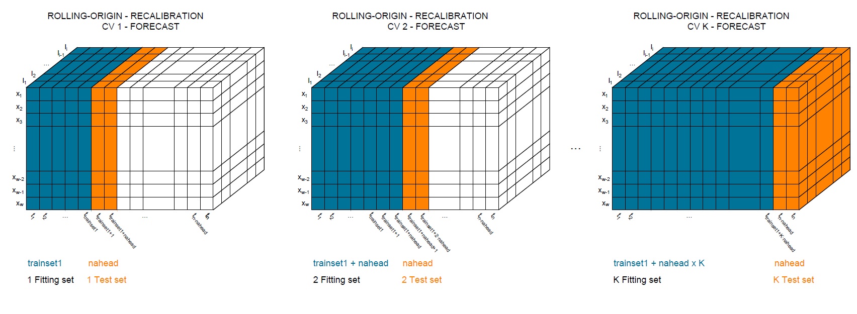
In the package, to apply this technique the users must provided a value of trainset1 higher than two (to meet with the minimum time-series size), and fixed_train_origin = TRUE (default value), independently of the assigned value of nahead.
There are different resampling techniques that can be applied based on the values of trainset1 and nahead.
Indeed, when nahead = 1 a Leave-One-Out-Cross-Validation (LOOCV) with RO-recalibration will be applied.
Independently, of the number of periods in the first train set (trainset1).
When, nahead and trainset1 are equal a K-Fold-Cross-Validation (LOOCV) with RO-recalibration will be applied.
For the rest values of nahead and trainset1 a standard time-series CV technique will be implemented.
Rolling-Window (RW) evaluation The approach is very similar to the RO-recalibration, but maintaining the training set size constant at each forecast/iteration. Maintaining the chronological order in each forecast, the training set adds the previous. projected periods of the test set and discards the earliest observations, as can be seen in the next Figure.
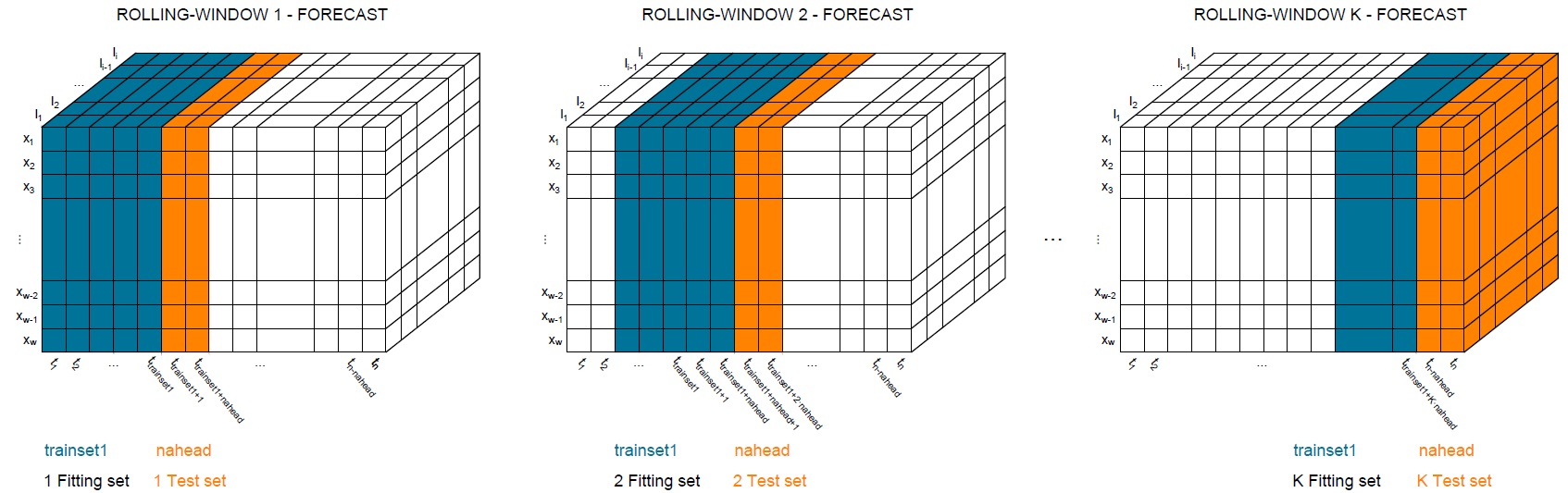
To apply this technique, the multipopulation_cv() function requires that fixed_train_origin = c(FALSE, "add_remove1"), regardless of the values of nahead and trainset1.
Equally as in RO-recalibration, LOOCV, and k-fold can be applied with nahead = 1, or nahead equals to trainset1, respectively, but keeping the training set constant through the iterations.
Additionally, the common time-series CV approach can be applied for different values of nahead and trainset1.
When fixed_train_origin = FALSE, at each iteration the training set adds the next nahead periods and discards the oldest keeping the training set size constant.
While fixed_train_origin = "add_remove1", at every iteration the training set only incorporates the next period ahead and discards only the latest period; maintaining the length of the training set constant and allowing to assess the forecasting accuracy of the mortality models in the long and medium term with different periods.
It should be mentioned that this function is developed for cross-validation the forecasting accuracy of several populations. However, in case you only consider one population, the function will forecast the Lee-Carter model for one population. To test the forecasting accuracy of the selected model, the function provides five different measures: SSE, MSE, MAE, MAPE or All of them. This measure of accuracy will be provided in different ways: a total measure, among ages considered, among populations and among projected blocked (periods). Depending on how you want to check the forecasting accuracy of the model you could select one or other. In this case, the measures will be obtained using the mortality rates in the normal scale as recommended by Santolino (2023) against the log scale.
Usage
multipopulation_cv(
  qxt,
  model = c("additive"),
  periods,
  ages,
  nPop,
  lxt = NULL,
  ktmethod = c("arima010"),
  order = NULL,
  nahead,
  trainset1,
  fixed_train_origin = TRUE,
  measures = c("SSE", "MSE", "MAE", "MAPE", "All"),
  ...
)
Arguments
qxt |
mortality rates used to fit the multi-population mortality models. These rates can be provided in the matrix or in a data.frame. |
model |
multi-population mortality model chosen to fit the mortality rates c(" |
periods |
number of years considered in the fitting in a vector way c( |
ages |
vector with the ages considered in the fitting. If the mortality rates provide from an abridged life tables, it is necessary to provide a vector with the ages, see the example. |
nPop |
number of population considered for fitting. |
lxt |
survivor function considered for every population, not necessary to provide. |
ktmethod |
method used to forecast the value of the trend parameter can choose among different ARIMA processes c(" |
order |
a vector or matrix (only when the |
nahead |
is a vector specifying the number of periods to forecast |
trainset1 |
is a vector with the periods for the first training set. This value must be greater than 2 to meet the minimum time series size (Hyndman and Khandakar, 2008). |
fixed_train_origin |
option to select whether the origin in the first train set is fixed or not. The default value is |
measures |
choose the non-penalized measure of forecasting accuracy that you want to use; c(" |
... |
additional arguments depending on the |
Value
An object of the class MultiCv including a list with different components of the cross-validation process:
-
axparameter that captures the average shape of the mortality curve in all considered populations. -
bxparameter that explains the age effect x with respect to the general trendktin the mortality rates of all considered populations. -
kt.fittedobtained values for the tendency behavior captured bykt. -
kt.futurefuture values ofktfor every iteration in the cross-validation. -
kt.arimathe ARIMA selected for eachkttime series. -
kt.orderorder of the components in the ARIMA models used for the trend parameters in every iteration. -
ktmethodmethod selected to forecast the value ofkt; the user can choose among different options; c("arimapdq", "arima010", "arimauser"). -
Iiparameter that captures the differences in the pattern of mortality in any region i with respect to Region 1. -
formulamulti-population mortality formula used to fit the mortality rates. -
modelprovided the model selected in every case. -
nPopprovided number of populations to fit the periods. -
qxt.crudecorresponds to the crude mortality rates. These crude rate are directly obtained by dividing the number of registered deaths by the number of those initially exposed to the risk for age x, period t and in each region i. -
qxt.futurefuture mortality rates estimated with the multi-population mortality model. -
logit.qxt.futurefuture mortality rates in logit way estimated with the multi-population mortality model. -
meas_agesmeasure of forecasting accuracy through the ages of the study. -
meas_periodsfutmeasure of forecasting accuracy in every forecasting period(s) of the study. -
meas_popmeasure of forecasting accuracy through the populations considered in the study. -
meas_totala global measure of forecasting accuracy through the ages, periods and populations of the study. -
warn_msgsvector with the populations where the model has not converged.
References
Atance, D., Debon, A., and Navarro, E. (2020). A comparison of forecasting mortality models using resampling methods. Mathematics 8(9): 1550.
Bergmeir, C. & Benitez, J.M. (2012) On the use of cross-validation for time series predictor evaluation. Information Sciences, 191, 192–
Carter, L.R. and Lee, R.D. (1992). Modeling and forecasting US sex differentials in mortality. International Journal of Forecasting, 8(3), 393–411.
Debon, A., & Atance, D. (2022). Two multi-population mortality models: A comparison of the forecasting accuracy with resampling methods. in Contributions to Risk Analysis: Risk 2022. Fundacion Mapfre
Debon, A., Montes, F., & Martinez-Ruiz, F. (2011). Statistical methods to compare mortality for a group with non-divergent populations: an application to Spanish regions. European Actuarial Journal, 1, 291-308.
Lee, R.D. & Carter, L.R. (1992). Modeling and forecasting US mortality. Journal of the American Statistical Association, 87(419), 659–671.
Li, N. and Lee, R.D. (2005). Coherent mortality forecasts for a group of populations: An extension of the Lee-Carter method. Demography, 42(3), 575–594.
Russolillo, M., Giordano, G., & Haberman, S. (2011). Extending the Lee–Carter model: a three-way decomposition. Scandinavian Actuarial Journal, 96-117.
Santolino, M. (2023). Should Selection of the Optimum Stochastic Mortality Model Be Based on the Original or the Logarithmic Scale of the Mortality Rate?. Risks, 11(10), 170.
See Also
fitLCmulti, forecast.fitLCmulti,
plot.fitLCmulti, plot.forLCmulti,
MeasureAccuracy.
Examples
#The example takes more than 5 seconds because they include
#several cross-validation methods and hence all the processes are included in "donttest".

#We present a cross-validation method for spanish male regions using:

ages <- c(0, 1, 5, 10, 15, 20, 25, 30, 35, 40,
         45, 50, 55, 60, 65, 70, 75, 80, 85, 90)
library(gnm)
library(forecast)
library(StMoMo)

#1. FIXED-ORIGIN -- using the ACFM nahead + trainset1 = periods;
#fixed_train_origin = TRUE (defualt value)
ho_Spainmales_addit <- multipopulation_cv(qxt = SpainRegions$qx_male,
                                         model = c("ACFM"),
                                         periods =  c(1991:2020), ages = c(ages),
                                         nPop = 18, lxt = SpainRegions$lx_male,
                                         nahead = 5,
                                         trainset1 = 25,
                                         ktmethod = c("arimapdq"),
                                         measures = c("SSE"))
ho_Spainmales_addit

#Once, we have run the function we can check the result in different ways:
ho_Spainmales_addit$meas_ages
ho_Spainmales_addit$meas_periodsfut
ho_Spainmales_addit$meas_pop
ho_Spainmales_addit$meas_total

#2. Let's continue with a RO-recalibration,
#(fixed_train_origin = TRUE (defualt value))
#where we have implemented three main CV techniques:
#2.1. Leave-One-Out-Cross-Validation (LOOCV) RO-recalibration when nahead = 1;
#(independently the number of periods blocked for the first train set; trainset1"
loocv_Spainmales_addit <- multipopulation_cv(qxt = SpainRegions$qx_male,
                                         model = c("additive"),
                                         periods =  c(1991:2020), ages = c(ages),
                                         nPop = 18, lxt = SpainRegions$lx_male,
                                         nahead = 1, trainset1 = 10,
                                         ktmethod = c("arimapdq"),
                                         measures = c("SSE"))
loocv_Spainmales_addit

#Once, we have run the function we can check the result in different ways:
loocv_Spainmales_addit$meas_ages
loocv_Spainmales_addit$meas_periodsfut
loocv_Spainmales_addit$meas_pop
loocv_Spainmales_addit$meas_total

#2.2. K-Fold-CV RO-recalibration when nahead = trainset1
kfoldcv_Spainmales_addit <- multipopulation_cv(qxt = SpainRegions$qx_male,
                                         model = c("additive"),
                                         periods =  c(1991:2020), ages = c(ages),
                                         nPop = 18, lxt = SpainRegions$lx_male,
                                         nahead = 5, trainset1 = 5,
                                         ktmethod = c("arimapdq"),
                                         measures = c("SSE"))
kfoldcv_Spainmales_addit

#Once, we have run the function we can check the result in different ways:
kfoldcv_Spainmales_addit$meas_ages
kfoldcv_Spainmales_addit$meas_periodsfut
kfoldcv_Spainmales_addit$meas_pop
kfoldcv_Spainmales_addit$meas_total

#2.3. standard time-series CV
cv_Spainmales_addit <- multipopulation_cv(qxt = SpainRegions$qx_male,
                                         model = c("additive"),
                                         periods =  c(1991:2020), ages = c(ages),
                                         nPop = 18, lxt = SpainRegions$lx_male,
                                         nahead = 5, trainset1 = 10,
                                         fixed_train_origin = TRUE,
                                         ktmethod = c("arimapdq"),
                                         measures = c("SSE"))

cv_Spainmales_addit
#Once, we have run the function we can check the result in different ways:
cv_Spainmales_addit$meas_ages
cv_Spainmales_addit$meas_periodsfut
cv_Spainmales_addit$meas_pop
cv_Spainmales_addit$meas_total

#3. RW-evaluation (fixed_train_origin = c(FALSE, "add_remove1"))
#3.1. fixed_train_origin = TRUE (The default value)
#In this case, the previous processes (Fixed-Origin or RO-recalibration)
#3.2. fixed_train_origin = FALSE
#where the origin in the training set is moved "nahead" period ahead in every iteration.
#This process allows to test the forecasting accuracy of "nahead" periods ahead
#keeping constant the size of the training and test set. As an example, we present
#three methods
#3.2.1. LOOCV
loocv_Spainmales_addit_rw <- multipopulation_cv(qxt = SpainRegions$qx_male,
                                         model = c("additive"),
                                         periods =  c(1991:2020), ages = c(ages),
                                         nPop = 18, lxt = SpainRegions$lx_male,
                                         nahead = 1, trainset1 = 10,
                                         fixed_train_origin = FALSE,
                                         ktmethod = c("arimapdq"),
                                         measures = c("SSE"))

loocv_Spainmales_addit_rw

#Once, we have run the function we can check the result in different ways:
loocv_Spainmales_addit_rw$meas_ages
loocv_Spainmales_addit_rw$meas_periodsfut
loocv_Spainmales_addit_rw$meas_pop
loocv_Spainmales_addit_rw$meas_total

#3.2.2. K-Fold-CV
kfoldcv_Spainmales_addit_rw <- multipopulation_cv(qxt = SpainRegions$qx_male,
                                         model = c("additive"),
                                         periods =  c(1991:2020), ages = c(ages),
                                         nPop = 18, lxt = SpainRegions$lx_male,
                                         nahead = 5, trainset1 = 5,
                                         fixed_train_origin = FALSE,
                                         ktmethod = c("arimapdq"),
                                         measures = c("SSE"))

kfoldcv_Spainmales_addit_rw

#Once, we have run the function we can check the result in different ways:
kfoldcv_Spainmales_addit$meas_ages
kfoldcv_Spainmales_addit$meas_periodsfut
kfoldcv_Spainmales_addit$meas_pop
kfoldcv_Spainmales_addit$meas_total

#3.2.3. standard time-series CV
cv_Spainmales_addit_rw <- multipopulation_cv(qxt = SpainRegions$qx_male,
                                         model = c("additive"),
                                         periods =  c(1991:2020), ages = c(ages),
                                         nPop = 18, lxt = SpainRegions$lx_male,
                                         nahead = 5, trainset1 = 10,
                                         fixed_train_origin = FALSE,
                                         ktmethod = c("arimapdq"),
                                         measures = c("SSE"))

cv_Spainmales_addit_rw

#Once, we have run the function we can check the result in different ways:
cv_Spainmales_addit_rw$meas_ages
cv_Spainmales_addit_rw$meas_periodsfut
cv_Spainmales_addit_rw$meas_pop
cv_Spainmales_addit_rw$meas_total

#3.3  RW-evaluation (fixed_train_origin = c("add_remove1"))
#where the origin in the training set is moved 1 period ahead in every iteration,
#adding the next period and removing the last period in the trainset.
#This process allows to test the forecasting accuracy of "nahead" periods ahead
#modifying the origin in the training set by 1.
#When "nahead" = 1 --- we will have a loocv equally as in the previous process,
#while using a different value of 1 for "nahead" we will test the forecasting
#accuracy of the model in "nahead" periods:
cv_Spainmales_addit_rw1 <- multipopulation_cv(qxt = SpainRegions$qx_male,
                                         model = c("additive"),
                                         periods =  c(1991:2020), ages = c(ages),
                                         nPop = 18, lxt = SpainRegions$lx_male,
                                         nahead = 5, trainset1 = 15,
                                         fixed_train_origin = "add_remove1",
                                         ktmethod = c("arimapdq"),
                                         measures = c("SSE"))
cv_Spainmales_addit_rw1

#Once, we have run the function we can check the result in different ways:
cv_Spainmales_addit_rw1$meas_ages
cv_Spainmales_addit_rw1$meas_periodsfut
cv_Spainmales_addit_rw1$meas_pop
cv_Spainmales_addit_rw1$meas_total
Function to plot the parameters of the multi-population mortality models
Description
R function to plot the parameters for the additive (Debon et al., 2011), multiplicative (Russolillo et al., 2011), common-factor (CFM) (Carter and Lee, 1992), Joint-k (Carter and Lee, 1992), and augmented-common factor (ACFM) (Li and Lee, 2005) multi-Population mortality model. It should be mentioned that in case that this function is developed for fitting several populations. However, in case you only consider one population, the function will fit the one-population Lee-Carter model (Lee and Carter, 1992).
Usage
## S3 method for class 'fitLCmulti'
plot(x, ...)
Arguments
x |
|
... |
additional arguments to show in the plot appearance. |
Value
plot the different parameters for the multi-population mortality models ax, bx, kt and Ii. This function is valid for both approaches Additive and Multiplicative multi-population mortality models.
References
Carter, L.R. and Lee, R.D. (1992). Modeling and forecasting US sex differentials in mortality. International Journal of Forecasting, 8(3), 393–411.
Debon, A., Montes, F., & Martinez-Ruiz, F. (2011). Statistical methods to compare mortality for a group with non-divergent populations: an application to Spanish regions. European Actuarial Journal, 1, 291-308.
Lee, R.D. & Carter, L.R. (1992). Modeling and forecasting US mortality. Journal of the American Statistical Association, 87(419), 659–671.
Li, N. and Lee, R.D. (2005). Coherent mortality forecasts for a group of populations: An extension of the Lee-Carter method. Demography, 42(3), 575–594.
Russolillo, M., Giordano, G., & Haberman, S. (2011). Extending the Lee–Carter model: a three-way decomposition. Scandinavian Actuarial Journal, 2011(2), 96-117.
Villegas, A. M., Haberman, S., Kaishev, V. K., & Millossovich, P. (2017). A comparative study of two-population models for the assessment of basis risk in longevity hedges. ASTIN Bulletin, 47(3), 631-679.
See Also
fitLCmulti, forecast.fitLCmulti,
plot.forLCmulti, multipopulation_cv
Examples
#The example takes more than 5 seconds because it includes
#several fitting and forecasting process and hence all
#the process is included in donttest

#First, we present the data that we are going to use
SpainRegions
ages <- c(0, 1, 5, 10, 15, 20, 25, 30, 35, 40, 45, 50, 55, 60, 65, 70, 75, 80, 85, 90)

library(gnm)
library(forecast)
#1. ADDITIVE MULTI-POPULATION MORTALITY MODEL
#In the case, the user wants to fit the additive multi-population mortality model
additive_Spainmales <- fitLCmulti(model = "additive",
                              qxt = SpainRegions$qx_male,
                              periods = c(1991:2020),
                              ages = c(ages),
                              nPop = 18,
                              lxt = SpainRegions$lx_male)

additive_Spainmales

#If the user does not provide the model inside the function fitLCmult()
#the multi-population mortality model applied will be additive one.

#Once, we have fit the data, it is possible to see the ax, bx, kt, and Ii
#provided parameters for the fitting.
plot(additive_Spainmales)

#2. MULTIPLICATIVE MULTI-POPULATION MORTALITY MODEL
#In the case, the user wants to fit the multiplicative multi-population mortality model
multiplicative_Spainmales <- fitLCmulti(model = "multiplicative",
                              qxt = SpainRegions$qx_male,
                              periods = c(1991:2020),
                              ages = c(ages),
                              nPop = 18,
                              lxt = SpainRegions$lx_male)

multiplicative_Spainmales

#Once, we have fit the data, it is possible to see the ax, bx, kt, and It
#provided parameters for the fitting.
plot(multiplicative_Spainmales)

#3. COMMON-FACTOR MULTI-POPULATION MORTALITY MODEL
#In the case, the user wants to fit the common-factor multi-population mortality model
cfm_Spainmales <- fitLCmulti(model = "CFM",
                             qxt = SpainRegions$qx_male,
                             periods = c(1991:2020),
                             ages = c(ages),
                             nPop = 18,
                             lxt = SpainRegions$lx_male)

cfm_Spainmales

#Once, we have fit the data, it is possible to see the ax, bx, kt, and It
#provided parameters for the fitting.
plot(cfm_Spainmales)

#4. JOINT-K MULTI-POPULATION MORTALITY MODEL
#In the case, the user wants to fit the augmented-common-factor multi-population mortality model
jointk_Spainmales <- fitLCmulti(model = "joint-K",
                                qxt = SpainRegions$qx_male,
                                periods = c(1991:2020),
                                ages = c(ages),
                                nPop = 18,
                                lxt = SpainRegions$lx_male)

jointk_Spainmales

#Once, we have fit the data, it is possible to see the ax, bx, kt, and It
#provided parameters for the fitting.
plot(jointk_Spainmales)

#5. AUGMENTED-COMMON-FACTOR MULTI-POPULATION MORTALITY MODEL
#In the case, the user wants to fit the augmented-common-factor multi-population mortality model
acfm_Spainmales <- fitLCmulti(model = "ACFM",
                              qxt = SpainRegions$qx_male,
                              periods = c(1991:2020),
                              ages = c(ages),
                              nPop = 18,
                              lxt = SpainRegions$lx_male)

acfm_Spainmales

#Once, we have fit the data, it is possible to see the ax, bx, kt, and It
#provided parameters for the fitting.
plot(acfm_Spainmales)

#6. LEE-CARTER FOR SINGLE-POPULATION
#As we mentioned in the details of the function, if we only provide the data
#from one-population the function fitLCmulti()
#will fit the Lee-Carter model for single populations.
LC_Spainmales <- fitLCmulti(qxt = SpainNat$qx_male,
                              periods = c(1991:2020),
                              ages = ages,
                              model = "additive",
                              nPop = 1)

LC_Spainmales

#Once, we have fit the data, it is possible to see the ax, bx, and kt
#parameters provided for the single version of the LC.
plot(LC_Spainmales)
Function to plot the parameters of the multi-population mortality models
Description
Function to plot different results of the forecasting process of multi-population mortality models, five different options which are obtained using the forecast.fitLCmulti() function.
In fact, the function will show the trend parameters kt fitted for the in-sample periods and its forecast results. Similarly, the behavior of the logit mortality rate for the mean in-sample age and the out-of-sample forecast will be shown for all the populations considered.
It should be mentioned that this function is developed for fitting several populations.
However, in case you only consider one population, the function will show the single population version of the Lee-Carter model, the classical one.
Usage
## S3 method for class 'forLCmulti'
plot(x, ...)
Arguments
x |
|
... |
additional arguments to show in the plot appearance. |
Value
plot the trend parameter kt fitted for the in-sample periods and its forecast results for the multi-population mortality models. Similarly, the behavior of the logit mortality rate for the mean in-sample age and the out-of-sample forecast will be shown for all the populations considered.
References
Carter, L.R. and Lee, R.D. (1992). Modeling and forecasting US sex differentials in mortality. International Journal of Forecasting, 8(3), 393–411.
Debon, A., Montes, F., & Martinez-Ruiz, F. (2011). Statistical methods to compare mortality for a group with non-divergent populations: an application to Spanish regions. European Actuarial Journal, 1, 291-308.
Lee, R.D. & Carter, L.R. (1992). Modeling and forecasting US mortality. Journal of the American Statistical Association, 87(419), 659–671.
Li, N. and Lee, R.D. (2005). Coherent mortality forecasts for a group of populations: An extension of the Lee-Carter method. Demography, 42(3), 575–594.
Russolillo, M., Giordano, G., & Haberman, S. (2011). Extending the Lee–Carter model: a three-way decomposition. Scandinavian Actuarial Journal, 2011(2), 96-117.
Villegas, A. M., Haberman, S., Kaishev, V. K., & Millossovich, P. (2017). A comparative study of two-population models for the assessment of basis risk in longevity hedges. ASTIN Bulletin, 47(3), 631-679.
See Also
fitLCmulti, forecast.fitLCmulti,
plot.fitLCmulti,
multipopulation_cv
Examples
#The example takes more than 5 seconds because it includes
#several fitting and forecasting process and hence all
#the process is included in donttest

#First, we present the data that we are going to use
SpainRegions
ages <- c(0, 1, 5, 10, 15, 20, 25, 30, 35, 40, 45, 50, 55, 60, 65, 70, 75, 80, 85, 90)

library(gnm)
library(forecast)
#1. ADDITIVE MULTI-POPULATION MORTALITY MODEL
#In the case, the user wants to fit the additive multi-population mortality model
additive_Spainmales <- fitLCmulti(model = "additive",
                              qxt = SpainRegions$qx_male,
                              periods = c(1991:2020),
                              ages = c(ages),
                              nPop = 18,
                              lxt = SpainRegions$lx_male)

additive_Spainmales

#If the user does not provide the model inside the function fitLCmult()
#the multi-population mortality model applied will be additive one.

#Once, we have fit the data, it is possible to see the ax, bx, kt, and Ii
#provided parameters for the fitting.
plot(additive_Spainmales)

#Once, we have fit the data, it is possible to forecast the multipopulation
#mortality model several years ahead, for example 10, as follows:
fut_additive_Spainmales <- forecast(object = additive_Spainmales, nahead = 10,
                                    ktmethod = "arimapdq")

fut_additive_Spainmales
#Once the data have been adjusted, it is possible to display the fitted kt and
#its out-of-sample forecasting. In addition, the function shows
#the logit mortality adjusted in-sample and projected out-of-sample
#for the mean age of the data considered in all populations.
plot(fut_additive_Spainmales)

#2. MULTIPLICATIVE MULTI-POPULATION MORTALITY MODEL
#In the case, the user wants to fit the multiplicative multi-population mortality model
multiplicative_Spainmales <- fitLCmulti(model = "multiplicative",
                              qxt = SpainRegions$qx_male,
                              periods = c(1991:2020),
                              ages = c(ages),
                              nPop = 18,
                              lxt = SpainRegions$lx_male)

multiplicative_Spainmales

#Once, we have fit the data, it is possible to see the ax, bx, kt, and It
#provided parameters for the fitting.
plot(multiplicative_Spainmales)

#Once, we have fit the data, it is possible to forecast the multipopulation
#mortality model several years ahead, for example 10, as follows:
fut_multi_Spainmales <- forecast(object = multiplicative_Spainmales, nahead = 10,
                                 ktmethod = "arimapdq")

fut_multi_Spainmales
#Once the data have been adjusted, it is possible to display the fitted kt and
#its out-of-sample forecasting. In addition, the function shows
#the logit mortality adjusted in-sample and projected out-of-sample
#for the mean age of the data considered in all populations.
plot(fut_multi_Spainmales)

#3. COMMON-FACTOR MULTI-POPULATION MORTALITY MODEL
#In the case, the user wants to fit the common-factor multi-population mortality model
cfm_Spainmales <- fitLCmulti(model = "CFM",
                             qxt = SpainRegions$qx_male,
                             periods = c(1991:2020),
                             ages = c(ages),
                             nPop = 18,
                             lxt = SpainRegions$lx_male)

cfm_Spainmales

#Once, we have fit the data, it is possible to see the ax, bx, kt, and It
#provided parameters for the fitting.
plot(cfm_Spainmales)

#Once, we have fit the data, it is possible to forecast the multipopulation
#mortality model several years ahead, for example 10.
#In this case, we apply another ktmethod = arimauser which implies to specify
#by the user the order of the trend parameters as follows:
fut_cfm_Spainmales <- forecast(object = cfm_Spainmales, nahead = 10,
                               ktmethod = "arimauser", order = c(0,1,0))

fut_cfm_Spainmales
#Once the data have been adjusted, it is possible to display the fitted kt and
#its out-of-sample forecasting. In addition, the function shows
#the logit mortality adjusted in-sample and projected out-of-sample
#for the mean age of the data considered in all populations.
plot(fut_cfm_Spainmales)

#4. AUGMENTED-COMMON-FACTOR MULTI-POPULATION MORTALITY MODEL
#In the case, the user wants to fit the augmented-common-factor multi-population mortality model
acfm_Spainmales <- fitLCmulti(model = "ACFM",
                              qxt = SpainRegions$qx_male,
                              periods = c(1991:2020),
                              ages = c(ages),
                              nPop = 18,
                              lxt = SpainRegions$lx_male)

acfm_Spainmales

#Once, we have fit the data, it is possible to see the ax, bx, kt, and It
#provided parameters for the fitting.
plot(acfm_Spainmales)

#Once, we have fit the data, it is possible to forecast the multipopulation
#mortality model several years ahead, for example 10, as follows:
fut_acfm_Spainmales <- forecast(object = acfm_Spainmales, nahead = 10,
                               ktmethod = "arimapdq")

fut_acfm_Spainmales
#Once the data have been adjusted, it is possible to display the fitted kt and
#its out-of-sample forecasting. In addition, the function shows
#the logit mortality adjusted in-sample and projected out-of-sample
#for the mean age of the data considered in all populations.
plot(fut_acfm_Spainmales)

#5. JOINT-K MULTI-POPULATION MORTALITY MODEL
#In the case, the user wants to fit the joint-K multi-population mortality model
jointk_Spainmales <- fitLCmulti(model = "joint-K",
                                qxt = SpainRegions$qx_male,
                                periods = c(1991:2020),
                                ages = c(ages),
                                nPop = 18,
                                lxt = SpainRegions$lx_male)

jointk_Spainmales

#Once, we have fit the data, it is possible to see the ax, bx, kt, and It
#provided parameters for the fitting.
plot(jointk_Spainmales)

#Once, we have fit the data, it is possible to forecast the multipopulation
#mortality model several years ahead, for example 10, as follows:
fut_jointk_Spainmales <- forecast(object = jointk_Spainmales, nahead = 10,
                               ktmethod = "arimapdq")

fut_jointk_Spainmales
#Once the data have been adjusted, it is possible to display the fitted kt and
#its out-of-sample forecasting. In addition, the function shows
#the logit mortality adjusted in-sample and projected out-of-sample
#for the mean age of the data considered in all populations.
plot(fut_jointk_Spainmales)

#6. LEE-CARTER FOR SINGLE-POPULATION
#As we mentioned in the details of the function, if we only provide the data
#from one-population the function fitLCmulti()
#will fit the Lee-Carter model for single populations.
LC_Spainmales <- fitLCmulti(qxt = SpainNat$qx_male,
                              periods = c(1991:2020),
                              ages = ages,
                              model = "additive",
                              nPop = 1)

LC_Spainmales

#Once, we have fit the data, it is possible to see the ax, bx, and kt
#parameters provided for the single version of the LC.
plot(LC_Spainmales)

#Once, we have fit the data, it is possible to forecast the multipopulation
#mortality model several years ahead, for example 10, as follows:
fut_LC_Spainmales <- forecast(object = LC_Spainmales, nahead = 10,
                              ktmethod = "arimapdq")

#Once the data have been adjusted, it is possible to display the fitted kt and
#its out-of-sample forecasting. In addition, the function shows
#the logit mortality adjusted in-sample and projected out-of-sample
#for the mean age of the data considered in all populations.
plot(fut_LC_Spainmales)
regions
Description
Data from the Spanish region of Spain which are provided to plot an indicator. This dataset contains a plot with the information of Spain regions (geometry and name of every region).
Usage
regions
Format
A data frame with 600 rows and 9 columns with class "SpainRegionsData" including the following information
-
Codigoa vector containing the code of every region of Spain. -
Textoa vector containing the name of every region of Spain. -
Texto_Alta vector containing the long name of every region of Spain. -
Iia vector containing a possible value of one indicator to be shown. -
geometrythe dimension of every region of Spain. This vector allows to plot the regions of Spain.
Value
a plot with the Spain regions colored by the indicator provided.
References
Spanish National Institute of Statistics (INE) (2023). Tablas de mortalidad, metodologia. Technical report, Instituto Nacional de Estadistica
Examples
#The example takes more than 5 seconds because it includes
#several fitting and forecasting process and hence all
#the process is included in donttest

#In this case, we show the region dataset applying it to a multipopulation model.
#First, we present the dataset

regions

ages <- c(0, 1, 5, 10, 15, 20, 25, 30, 35, 40, 45, 50, 55, 60, 65, 70, 75, 80, 85, 90)

#Then, we fit the multiplicative model
library(gnm)
multiplicative_Spainmales <- fitLCmulti(model = "multiplicative",
                                        qxt = SpainRegions$qx_male,
                                        periods = c(1991:2020),
                                        ages = c(ages),
                                        nPop = 18,
                                        lxt = SpainRegions$lx_male)

multiplicative_Spainmales
library(sf)
#To show the values of the population indicator in the Spanish map.
SpainMap(regionvalue = multiplicative_Spainmales$Ii[2:18],
         main = c("Multiplicative for males"),
         name = c("Ii"))
Function to extract the resid from SVD
Description
This function uses the first d components of the singular value
decomposition in order to approximate a vector of model residuals by a
sum of d multiplicative terms, with the multiplicative
structure determined by two specified factors follows the SVD function by Turner et al. (2023).
For glm and gnm models from the gnm R-packages,
the matrix entries are weighted working residuals. The primary use of residSVD is to
generate good starting values for the parameters in Mult terms
in models to be fitted using gnm. In this case, we modified the function
in order to obtain good starting values for the multi-population mortality models.
Usage
residSVD2(model, fac1, fac2, d = 1)
Arguments
model |
object with na.action, residuals, and weights methods, e.g. objects inheriting from class |
fac1 |
first factor. |
fac2 |
second factor. |
d |
integer, the number of multiplicative terms to use in the approximation. |
Value
If d = 1, a numeric vector; otherwise a numeric matrix with d columns.
References
Turner, H., & Firth, D. (2023). Generalized nonlinear models in R: An overview of the gnm package. R package version 1.1-5. https://CRAN.R-project.org/package=gnm
See Also
fitLCmulti, forecast.fitLCmulti
multipopulation_cv, plot.fitLCmulti
plot.forLCmulti