Help for package HBV.IANIGLA

Type:

Package

Title:

Modular Hydrological Model

Version:

0.2.6

Date:

2022-11-23

Author:

Ezequiel Toum <etoum@mendoza-conicet.gob.ar>

Maintainer:

Ezequiel Toum <etoum@mendoza-conicet.gob.ar>

Description:

The HBV hydrological model (Bergström, S. and Lindström, G., (2015) <doi:10.1002/hyp.10510>) has been split in modules to allow the user to build his/her own model. This version was developed by the author in IANIGLA-CONICET (Instituto Argentino de Nivologia, Glaciologia y Ciencias Ambientales - Consejo Nacional de Investigaciones Cientificas y Tecnicas) for hydroclimatic studies in the Andes. HBV.IANIGLA incorporates routines for clean and debris covered glacier melt simulations.

License:

GPL (≥ 3)

Encoding:

UTF-8

LazyData:

true

Imports:

Rcpp

URL:

https://gitlab.com/ezetoum27/hbv.ianigla

BugReports:

https://gitlab.com/ezetoum27/hbv.ianigla/-/issues

Depends:

R (≥ 3.5.0)

LinkingTo:

Rcpp

RoxygenNote:

7.2.1

Suggests:

knitr, rmarkdown

VignetteBuilder:

knitr

NeedsCompilation:

yes

Packaged:

2022-11-23 13:08:41 UTC; eze

Repository:

CRAN

Date/Publication:

2022-11-23 23:50:02 UTC

Glacier discharge conceptual model

Description

Implement the conceptual water storage and release formulation for glacier runoff routing. The current model version follows the approach proposed by Stahl et al. (2008) (hereafter S08) for the Bridge River basin. Note that the bucket storage and release concepts for glacier runoff modeling are also described in Jansson et al. (2002).

Usage

Glacier_Disch(
       model,
       inputData,
       initCond,
       param
       )

Arguments

model

numeric integer with the model's choice. The current HBV.IANIGLA version only supports the S08 approach.

1:S08 glacier storage and release model.

inputData

numeric matrix with two columns:

Model 1

column_1: snow water equivalent above the glacier [mm/\Delta t]. The series can be obtained from the SnowGlacier_HBV function output.
column_2: melted snow + melted ice + rainfall [mm/\Delta t]. This series comes from the TotScal column in the SnowGlacier_HBV function output.

initCond

numeric value with the initial glacier reservoir water content SG [mm].

param

numeric vector with the following values:

Model 1 (S08)

KGmin: minimal outflow rate [1/\Delta t].
dKG: maximum outflow rate increase [1/\Delta t].
AG: scale factor [mm].

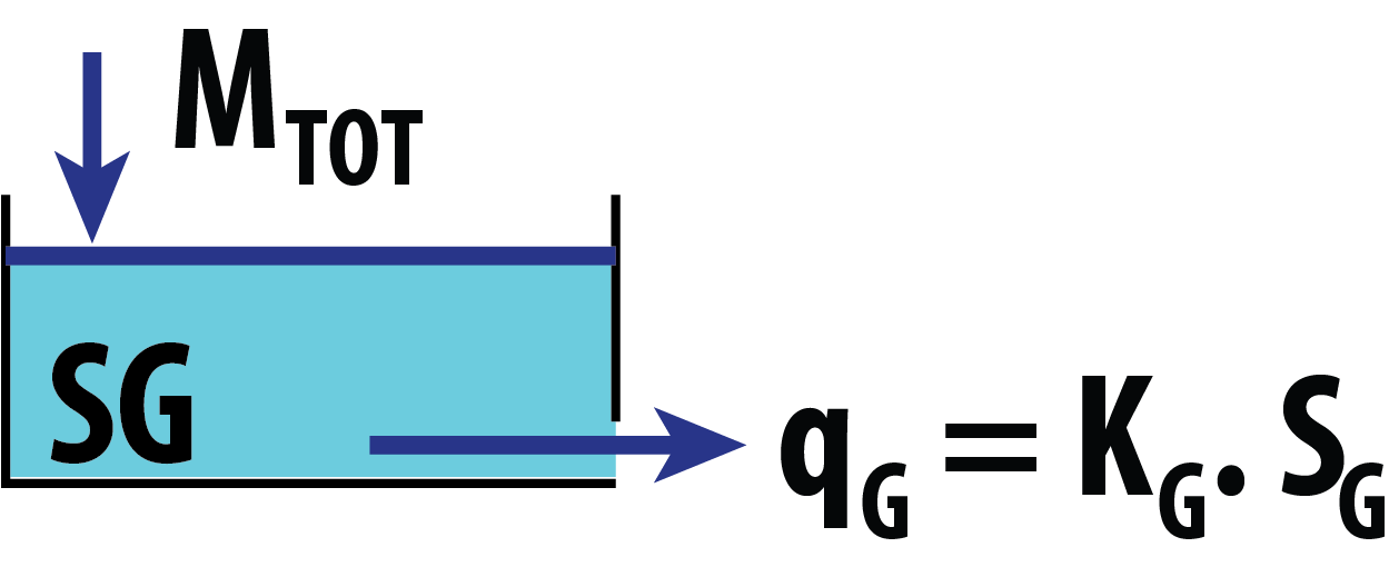
Value

Numeric matrix with the following columns:

Model 1 (S08)

Q: glacier discharge [mm/\Delta t].
SG: glacier's bucket water storage content series [1/\Delta t].

References

Jansson, P., Hock, R., Schneider, T., 2003. The concept of glacier storage: a review. J. Hydrol., Mountain Hydrology and Water Resources 282, 116–129. https://doi.org/10.1016/S0022-1694(03)00258-0

Stahl, K., Moore, R.D., Shea, J.M., Hutchinson, D., Cannon, A.J., 2008. Coupled modelling of glacier and streamflow response to future climate scenarios. Water Resour. Res. 44, W02422. https://doi.org/10.1029/2007WR005956

Examples

# The following is a toy example. I strongly recommend to see
# the package vignettes in order to improve your skills on HBV.IANIGLA

## Create an input data and run the module
DataMatrix <- cbind(
                    runif(n = 100, min = 0, max = 50),
                    runif(n = 100, min = 0, max = 200)
                    )

dischGl    <- Glacier_Disch(model = 1, inputData = DataMatrix,
                           initCond = 100, param = c(0.1, 0.9, 10))

Potential evapotranspiration models

Description

Calculate your potential evapotranspiration series. This module was design to provide a simple and straight forward way to calculate one of the inputs for the soil routine (to show how does it works), but for real world application I strongly recommend the use of the specialized Evapotranspiration package.

Usage

PET(
  model,
  hemis,
  inputData,
  elev,
  param
  )

Arguments

model

numeric value with model option:

1: Calder's model.

hemis

numeric value indicating the hemisphere:

1: southern hemisphere.
2: northern hemisphere.

inputData

numeric matrix with the following columns:

Calder's model

column_1: julian dates, e.g: as.matrix( c(1:365) ).

elev

numeric vector with the following values:

Calder's model

1: zref: the reference height where potential evapotranspiration or input data to calculate PET is known.
2: ztopo: target PET's topographic height.

param

numeric vector with the following values:

Calder's model

1: PET: climatological daily mean potential evapotranspiration [mm].
2: gradPET: evapotranspiration decrease gradient [mm/100 m].

Value

Numeric vector with the potential evapotranspiration series.

References

Calder, I.R., Harding, R.J., Rosier, P.T.W., 1983. An objective assessment of soil-moisture deficit models. J. Hydrol. 60, 329–355. https://doi.org/10.1016/0022-1694(83)90030-6

Examples

# The following is a toy example. I strongly recommend to see
# the package vignettes in order to improve your skills on HBV.IANIGLA

## Run the model for a year in the southern hemisphere
potEvap <- PET(model = 1,
               hemis = 1,
               inputData = as.matrix(1:365),
               elev = c(1000, 1500),
               param = c(4, 0.5))

Altitude gradient based precipitation models

Description

Extrapolate precipitation gauge measurements to another heights. In this package version you can use the classical linear gradient model or a modified version which sets a threshold altitude for precipitation increment (avoiding unreliable estimations).

Usage

Precip_model(
       model,
       inputData,
       zmeteo,
       ztopo,
       param
)

Arguments

model

numeric value with model option:

1: linear precipitation gradient (LP).
2: linear precipitation gradient with an upper threshold (LPM).

inputData

numeric vector with precipitation gauge series [mm/\Delta t].

zmeteo

numeric value indicating the altitude of the precipitation gauge [masl].

ztopo

numeric value with the target height [masl].

param

numeric vector with the following parameters:

1: precipitation gradient (gradP) [%/100m].

LPM

1: precipitation gradient (gradP) [%/100m].
2: threshold height. Precipitation does not increase when the altitude (ztopo) is higher than this parameter [masl].

Value

Numeric vector with the extrapolated precipitation series.

References

For some interesting work on precipitation gradients at catchment and synoptic scale see:

Immerzeel, W.W., Petersen, L., Ragettli, S., Pellicciotti, F., 2014. The importance of observed gradients of air temperature and precipitation for modeling runoff from a glacierized watershed in the Nepalese Himalayas. Water Resour. Res. 50, 2212–2226. https://doi.org/10.1002/2013WR014506

Viale, M., Nuñez, M.N., 2010. Climatology of Winter Orographic Precipitation over the Subtropical Central Andes and Associated Synoptic and Regional Characteristics. J. Hydrometeorol. 12, 481–507. https://doi.org/10.1175/2010JHM1284.1

Examples

# The following is a toy example. I strongly recommend to see
# the package vignettes in order to improve your skills on HBV.IANIGLA

## LP case
set.seed(369)

precLP <- Precip_model(model = 1, inputData = runif(n = 365, max = 30, min = 0),
                        zmeteo = 3000, ztopo = 4700, param = c(5))

## LPM case
set.seed(369)

precLPM <- Precip_model(model = 2, inputData = runif(n = 365, max = 30, min = 0),
                        zmeteo = 3000, ztopo = 4700, param = c(5, 4500))

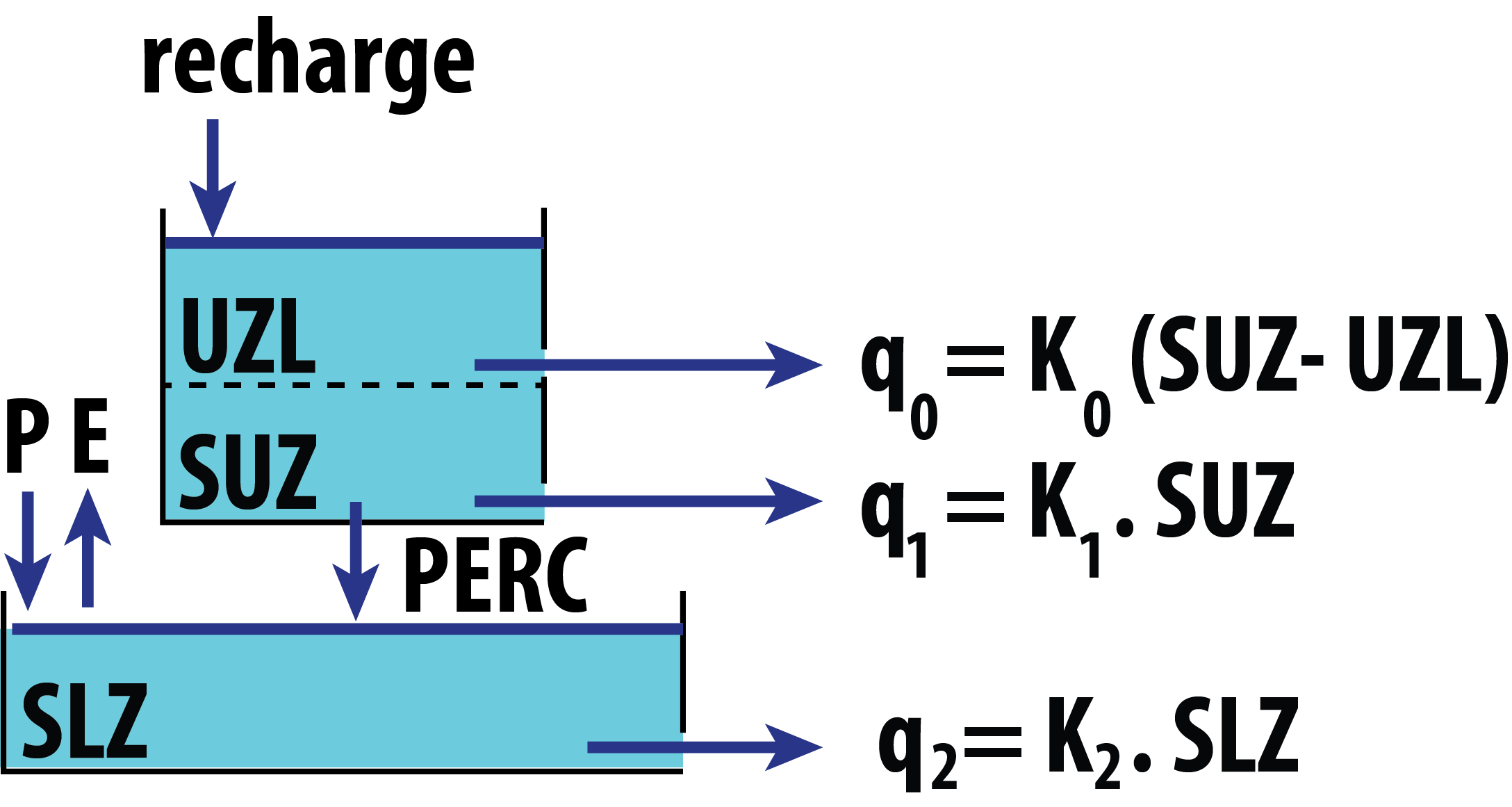
Routing bucket type models

Description

Implement one of the five different bucket formulations for runoff routing. The output of this function is the input series of the transfer function (UH).

Usage

Routing_HBV(
       model,
       lake,
       inputData,
       initCond,
       param
       )

Arguments

model

numeric integer indicating which reservoir formulation to use:

1: Three series of reservoirs. Lake option is allowed.
2: Two series of reservoirs. Lake option is allowed.
3: Two reservoirs and three outlets. Lake option is allowed.
4: One reservoir and two outlets. Lake is NOT allowed.
5: One reservoir and three outlets. Lake is NOT allowed.

lake

logical. A TRUE value will enable the lake option (only available on models 1, 2 and 3). When modeling a lake, HBV.IANIGLA considers that this water body exist on the bottom bucket, so you will also have to provide a lake evaporation and precipitation series in the inputData matrix.

inputData

numeric matrix with three columns (two of them depends on lake option).

column_1: effective runoff series [mm/\Delta T]. This is the output of the Soil_HBV module.
column_2: only if lake = TRUE. Precipitation series falling in the lake. When using it remember that the precipitation should be rescaled according to the relative area of the lake in the basin.
column_3: only if lake = TRUE. Lake's evaporation series. When using it remember that the precipitation should be rescaled according to the relative area of the lake in the basin.

initCond

numeric vector with the following initial state variables.

SLZ0: initial water content of the lower reservoir [mm]. This state variable is compulsory for all model options.
SUZ0: initial water content of the intermediate reservoir [mm]. This option does not make sense for models 4 and 5.
STZ0: initial water content of the upper reservoir [mm]. This option only make sense for model 1.

param

numeric vector. The length depends on the model's choice:

Model 1

K0: top bucket (STZ) storage constant [1/\Delta t].
K1: intermediate bucket (SUZ) storage constant [1/\Delta t].
K2: lower bucket (SLZ) storage constant [1/\Delta t].
UZL: maximum flux rate between STZ and SUZ [mm/\Delta t].
PERC: maximum flux rate between SUZ and SLZ [mm/\Delta t].

Model 2

K1: intermediate bucket (SUZ) storage constant [1/\Delta t].
K2: lower bucket (SLZ) storage constant [1/\Delta t].
PERC: maximum flux rate between SUZ and SLZ [mm/\Delta t].

Model 3

K0: top output (Q0) storage constant [1/\Delta t].
K1: intermediate bucket (SUZ) storage constant [1/\Delta t].
K2: lower bucket (SLZ) storage constant [1/\Delta t].
UZL: minimum water content of SUZ for supplying fast runoff (Q0) to the total reservoir discharge (Qg) [mm].
PERC: maximum flux rate between SUZ and SLZ [mm/\Delta t].

Model 4

K1: intermediate output (Q1) storage constant [1/\Delta t].
K2: lower bucket (SLZ) storage constant [1/\Delta t].
PERC: minimum water content of SLZ for supplying intermediate runoff (Q1) to the total reservoir discharge (Qg) [mm].

Model 5

K0: top output (Q0) storage constant [1/\Delta t].
K1: intermediate output (Q1) storage constant [1/\Delta t].
K2: lower bucket (SLZ) storage constant [1/\Delta t].
UZL: minimum water content of SLZ for supplying fast runoff (Q0) to the total reservoir discharge (Qg) [mm].
PERC: minimum water content of SLZ for supplying intermediate runoff (Q1) to the total reservoir discharge (Qg) [mm].

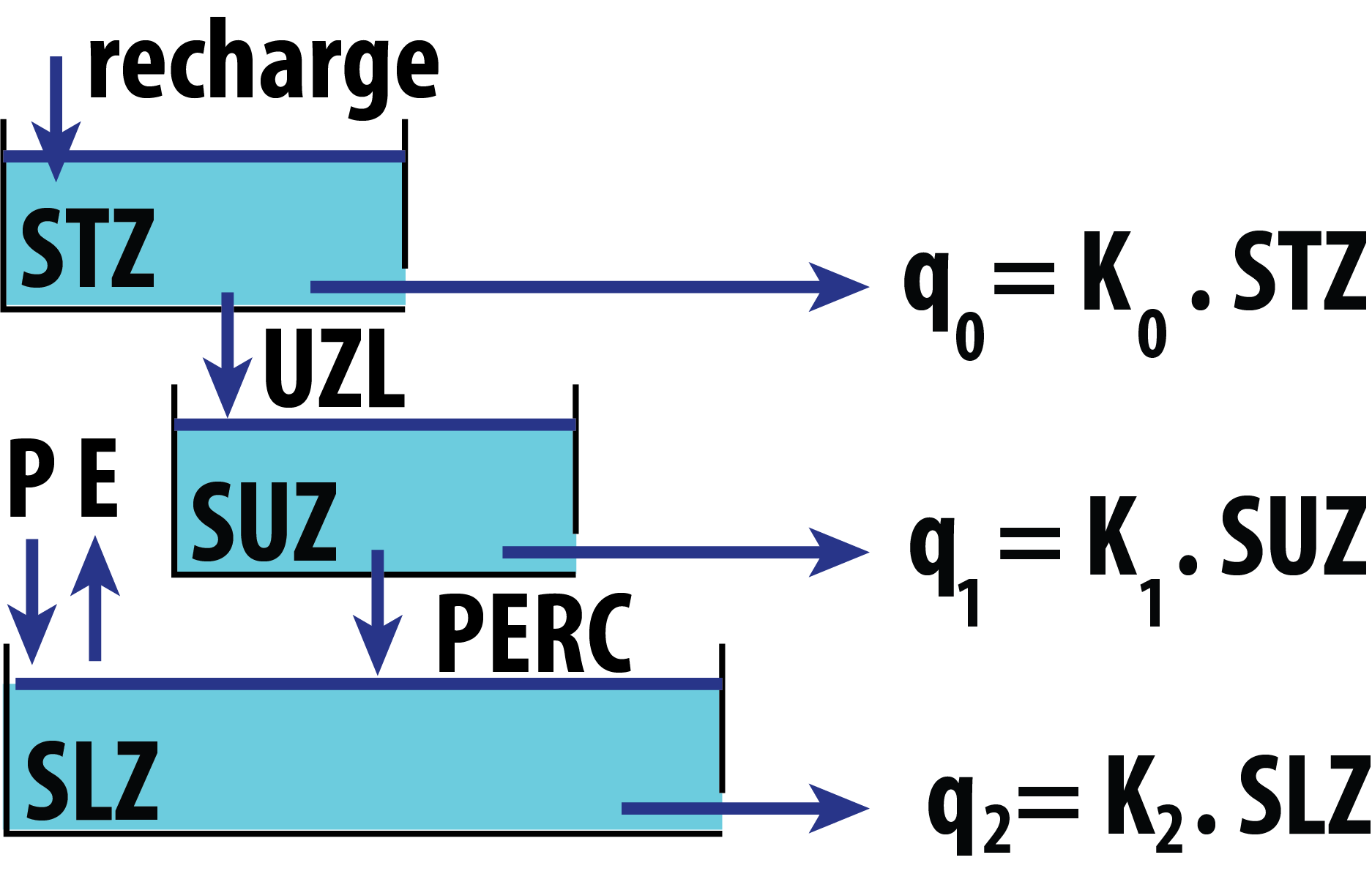
Value

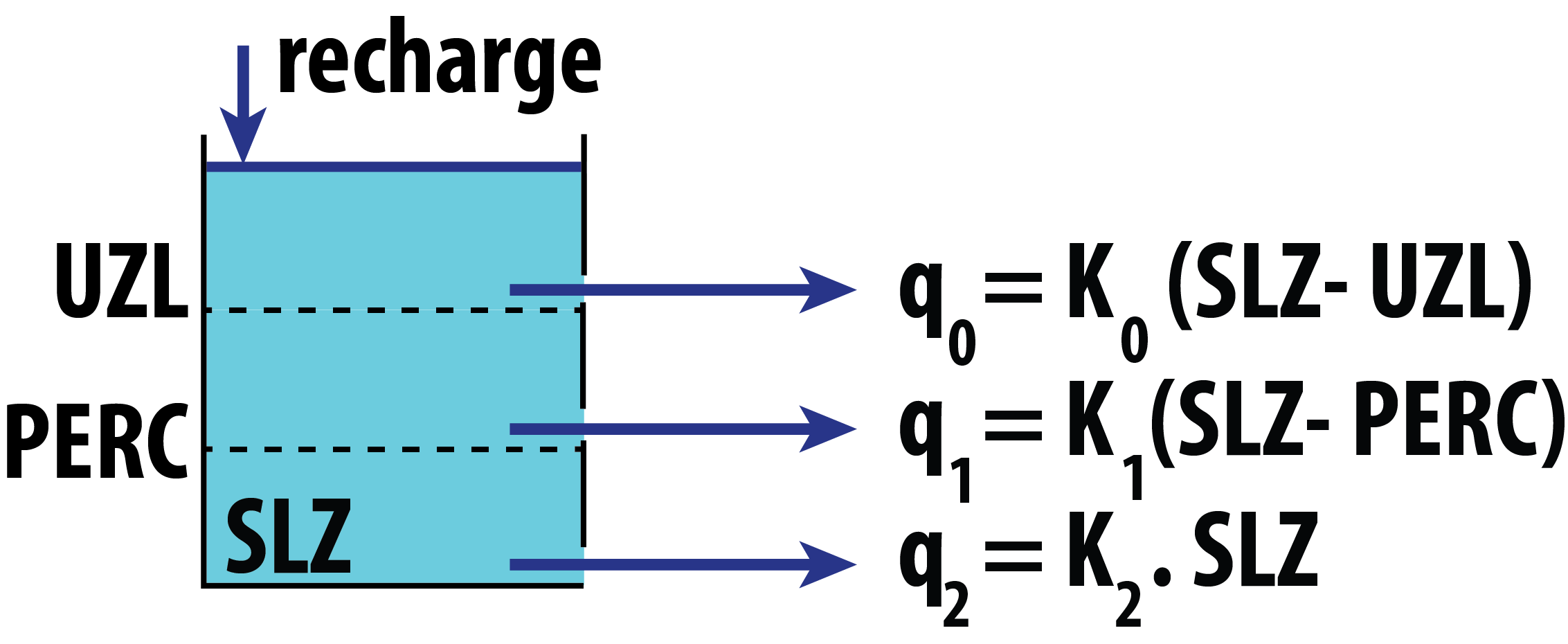
Numeric matrix with the following columns:

Model 1

Qg: total buckets output discharge [mm/\Delta t].
Q0: top bucket discharge [mm/\Delta t].
Q1: intermediate bucket discharge [mm/\Delta t].
Q2: lower bucket discharge [mm/\Delta t].
STZ: top reservoir storage [mm].
SUZ: intermediate reservoir storage [mm].
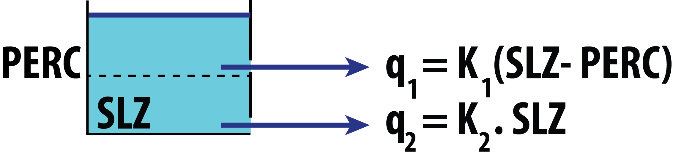
SLZ: lower reservoir storage [mm].

Model 2

Qg: total buckets output discharge [mm/\Delta t].
Q1: intermediate bucket discharge [mm/\Delta t].
Q2: lower bucket discharge [mm/\Delta t].
SUZ: intermediate reservoir storage [mm].
SLZ: lower reservoir storage [mm].

Model 3

Qg: total buckets output discharge [mm/\Delta t].
Q0: intermediate bucket fast discharge [mm/\Delta t].
Q1: intermediate bucket discharge [mm/\Delta t].
Q2: lower bucket discharge [mm/\Delta t].
SUZ: intermediate reservoir storage [mm].
SLZ: lower reservoir storage [mm].

Model 4

Qg: total buckets output discharge [mm/\Delta t].
Q1: lower bucket intermediate discharge [mm/\Delta t].
Q2: lower bucket discharge [mm/\Delta t].
SLZ: lower reservoir storage [mm].

Model 5

Qg: total buckets output discharge [mm/\Delta t].
Q0: lower bucket fast discharge [mm/\Delta t].
Q1: lower bucket intermediate discharge [mm/\Delta t].
Q2: lower bucket discharge [mm/\Delta t].
SLZ: lower reservoir storage [mm].

References

Bergström, S., Lindström, G., 2015. Interpretation of runoff processes in hydrological modelling—experience from the HBV approach. Hydrol. Process. 29, 3535–3545. https://doi.org/10.1002/hyp.10510

Beven, K.J., 2012. Rainfall - Runoff Modelling, 2 edition. ed. Wiley, Chichester.

Seibert, J., Vis, M.J.P., 2012. Teaching hydrological modeling with a user-friendly catchment-runoff-model software package. Hydrol Earth Syst Sci 16, 3315–3325. https://doi.org/10.5194/hess-16-3315-2012

Examples

# The following is a toy example. I strongly recommend to see
# the package vignettes in order to improve your skills on HBV.IANIGLA

## Case example with the first model
inputMatrix <- cbind(
                     runif(n = 200, max = 100, min = 0),
                     runif(n = 200, max = 50, min = 5),
                     runif(n = 100, max = 3, min = 1)
                     )

routeMod1   <- Routing_HBV(model = 1, lake = TRUE, inputData = inputMatrix,
                     initCond = c(10, 15, 20), param = c(0.1, 0.05, 0.001, 1, 0.8))

Snow and ice-melt models

Description

Allows you to simulate snow accumulation and melting processes using a temperature index approach. The function also incorporates options for clean and debris covered glacier surface mass balance simulations.

Usage

SnowGlacier_HBV(
       model,
       inputData,
       initCond,
       param
)

Arguments

model

numeric indicating which model you will use:

1: temperature index model.
2: temperature index model with a variable snow cover area as input data (as in the Snowmelt Runoff Model - SRM).
3: temperature index model with a variable glacier area as input data.

inputData

numeric matrix being columns the input variables. As in the whole package functions, NA_real_ values are forbidden. When speaking about model options we refer to the model argument.

Model 1:

column_1: air temperature series [°C/\Delta t].
column_2: precipitation series [mm/\Delta t].

Model 2:

column_1: air temperature [°C/\Delta t].
column_2: precipitation [mm/\Delta t].
column_3: snow cover area. Values between [0 ; 1] [-].

Model 3:

column_1: air temperature [°C/\Delta t].
column_2: precipitation [mm/\Delta t].
column_3: glacier cover area. This area values are relative to the total surface area of the basin [-].

initCond

numeric vector with the following values.

SWE0: initial snow water equivalent [mm].
numeric integer indicating the surface type. 1: clean ice; 2: soil; 3: debris-covered ice.
area of the glacier(s) (in the elevation band) relative to the basin; e.g.: 0.1 [-]. This option is required in Model 1 and Model 2 when surface is a glacier.

param

numeric vector with the following values:

SFCF: snowfall correction factor [-].
Tr: solid and liquid precipitation threshold temperature [ºC].
Tt: melt temperature [ºC].
fm: snowmelt factor [mm/°C.\Delta t].
fi: icemelt factor [mm/°C.\Delta t].
fic: debris-covered ice-melt factor [mm/°C.\Delta t].

Value

Numeric matrix with the following columns:

Model 1

** if surface is soil,

Prain: precip. as rainfall.
Psnow: precip. as snowfall.
SWE: snow water equivalent.
Msnow: melted snow.
Total: Prain + Msnow.

** if surface is ice,

Prain: precip. as rainfall.
Psnow: precip. as snowfall.
SWE: snow water equivalent.
Msnow: melted snow.
Mice: melted ice.
Mtot: Msnow + Mice.
Cum: Psnow - Mtot.
Total: Prain + Mtot.
TotScal: Total * initCond[3].

Model 2

** if surface is soil,

Prain: precip. as rainfall.
Psnow: precip. as snowfall.
SWE: snow water equivalent.
Msnow: melted snow.
Total: Prain + Msnow.
TotScal: Msnow * SCA + Prain.

** if surface is ice -> as in Model 1

Model 3

** if surface is soil -> as in Model 1

** if surface is ice,

Prain: precip. as rainfall.
Psnow: precip. as snowfall.
SWE: snow water equivalent.
Msnow: melted snow.
Mice: melted ice.
Mtot: Msnow + Mice.
Cum: Psnow - Mtot.
Total: Prain + Mtot.
TotScal: Total * inputData[i, 3].

References

DeWalle, D. R., & Rango, A. (2008). Principles of Snow Hydrology.

Parajka, J., Merz, R., Blöschl, G., 2007. Uncertainty and multiple objective calibration in regional water balance modelling: case study in 320 Austrian catchments. Hydrol. Process. 21, 435–446. https://doi.org/10.1002/hyp.6253

Examples

# The following is a toy example. I strongly recommend to see
# the package vignettes in order to improve your skills on HBV.IANIGLA

## Debris-covered ice
ObsTemp   <- sin(x = seq(0, 10*pi, 0.1))
ObsPrecip <- runif(n = 315, max = 50, min = 0)
ObsGCA    <- seq(1, 0.8, -0.2/314)

## Fine debris covered layer assumed. Note that the ice-melt factor is cumpulsory but harmless.
DebrisCovGlac <- SnowGlacier_HBV(model = 3,
                                 inputData = cbind(ObsTemp, ObsPrecip, ObsGCA),
                                 initCond = c(10, 3, 1),
                                 param = c(1, 1, 0, 3, 1, 6))

Empirical soil moisture routine

Description

This module allows you to account for actual evapotranspiration, abstractions, antecedent conditions and effective runoff. The formulation enables non linear relationships between soil box water input (rainfall plus snowmelt) and the effective runoff. This effective value is the input series to the routine function (Routing_HBV).

Usage

Soil_HBV(
       model,
       inputData,
       initCond,
       param
       )

Arguments

model

numeric integer suggesting one of the following options:

1: Classical HBV soil moisture routine.
2: HBV soil moisture routine with varying area. This option should be used with SnowGlacier_HBV's model 3.

inputData

numeric matrix with the following series

Model 1

column_1: Total = Prain + Msnow [mm/\Delta t]. This series comes from the output of the SnowGlacier_HBV module.
column_2: potential evapotranspiration [mm/\Delta t]. Since the package has a simple model (PET) to obtain this series I strongly recommend using the Evapotranspiration package.

Model 2

column_1: as in model 1.
column_2: as in model 1.
column_3 : relative soil area (ratio of soil surface over basin area). When the glacier area changes the soil does the same, so coherence between this two series should be seek.This value is used to scale the effective runoff accordingly (Rech column in the matrix output).

initCond

numeric vector with the following values:

initial soil water content [mm]. This is a model state variable and is internally used as first soil moisture value.
relative area [-]. Only needed when using model 1. This is the soil surface proportion relative to the catchment as a whole, so the values should never supersede one (1). This value is used to scale the effective runoff accordingly (Rech column in the matrix output).

param

numeric vector with the following values:

FC: fictitious soil field capacity [mm].
LP: parameter to get actual ET [-].
\beta: exponential value that allows for non-linear relations between soil box water input (rainfall plus snowmelt) and the effective runoff [-].

Value

Numeric matrix with the following columns:

Rech: recharge series [mm/\Delta t]. This is the input to the Routing_HBV module.
Eact: actual evapotranspiration series [mm/\Delta t].
SM: soil moisture series [mm/\Delta t].

References

Examples

# The following is a toy example. I strongly recommend to see
# the package vignettes in order to improve your skills on HBV.IANIGLA

# HBV soil routine with variable area
## Calder's model
potEvap <- PET(model = 1, hemis = 1, inputData = as.matrix(1:315), elev = c(1000, 1500),
              param = c(4, 0.5))

## Debris-covered ice
 ObsTemp   <- sin(x = seq(0, 10*pi, 0.1))
 ObsPrecip <- runif(n = 315, max = 50, min = 0)
 ObsGCA    <- seq(1, 0.8, -0.2/314)

## Fine debris covered layer assumed. Note that the ice-melt factor is cumpulsory but harmless.
DebrisCovGlac <- SnowGlacier_HBV(model = 3, inputData = cbind(ObsTemp, ObsPrecip, ObsGCA),
                                 initCond = c(10, 3, 1), param = c(1, 1, 0, 3, 1, 6))

## Soil routine
ObsSoCA     <- 1 - ObsGCA
inputMatrix <- cbind(DebrisCovGlac[ , 9], potEvap, ObsSoCA)

soil <- Soil_HBV(model = 2, inputData = inputMatrix, initCond = c(50), param = c(200, 0.5, 2))

Altitude gradient base air temperature models

Description

Extrapolate air temperature records to another heights. In this package version you can use the classical linear gradient model or a modified version which sets an upper altitudinal threshold air temperature decrement (avoiding unreliable estimations).

Usage

Temp_model(
       model,
       inputData,
       zmeteo,
       ztopo,
       param
)

Arguments

model

numeric value with model option:

1: linear air temperature gradient (LT).
2: linear air temperature gradient with an upper threshold (LTM).

inputData

numeric vector with air temperature record series [ºC/\Delta t].

zmeteo

numeric value indicating the altitude where the air temperature is recorded [masl].

ztopo

numeric value with the target height [masl].

param

numeric vector with the following parameters:

1: air temperature linear gradient (grad_t) [ºC/km].

LPM

1: air temperature linear gradient (grad_t) [ºC/km].
2: threshold height. Air temperature does not decrease when the altitude (ztopo) is higher than this value [masl].

Value

Numeric vector with the extrapolated air temperature series.

References

Examples

# The following is a toy example. I strongly recommend to see
# the package vignettes in order to improve your skills on HBV.IANIGLA

## simple linear model
airTemp <- Temp_model(
                      model = 1,
                      inputData = runif(200, max = 25, min = -10),
                      zmeteo = 2000, ztopo = 3500, param = c(-6.5)
                      )

Transfer function

Description

Use a triangular transfer function to adjust the timing of the simulated streamflow discharge. This module represents the runoff routing in the streams.

Usage

UH(
  model,
  Qg,
  param
  )

Arguments

model

numeric integer with the transfer function model. The current HBV.IANIGLA model only allows for a single option.

1: triangular function with a static base.

Qg

numeric vector with the water that gets into the stream. If you are not modeling glaciers is the output of the Routing_HBV module, otherwise, is the sum of the Routing_HBV output plus the glacier discharge coming from the Glacier_Disch module.

param

numeric vector with the following values,

Model 1

Bmax: base of the transfer function triangle [timestep].

Value

Numeric vector with the simulated streamflow discharge.

References

Parajka, J., Merz, R., & Blöschl, G. (2007). Uncertainty and multiple objective calibration in regional water balance modelling: Case study in 320 Austrian catchments. Hydrological Processes, 21(4), 435-446. https://doi.org/10.1002/hyp.6253

Examples

# The following is a toy example. I strongly recommend to see
# the package vignettes in order to improve your skills on HBV.IANIGLA

## Routing example
inputMatrix <- cbind(runif(n = 200, max = 100, min = 0), runif(n = 200, max = 50, min = 5),
                 runif(n = 100, max = 3, min = 1))

routeMod1   <- Routing_HBV(model = 1, lake = TRUE, inputData = inputMatrix,
                         initCond = c(10, 15, 20), param = c(0.1, 0.05, 0.001, 1, 0.8))

## UH
dischOut <- UH(model = 1, Qg = routeMod1[ , 1], param = 2.2)

Alerce's glacier data for modeling

Description

A dataset containing all necessary information to simulate a three year glacier surface mass balance. The ice body is located on Monte Tronador, nearby the border between Argentina and Chile in the Andes of Northern Patagonia. Alerce is a medium size mountain glacier with an area of about 2.33 km2 that ranges between 1629 and 2358 masl and it shows a SE aspect (IANIGLA-ING, 2018).

Usage

alerce_data

Format

A list with five elements

mass_balance: data frame with the estimated annual mass balance and the acceptable uncertainty bounds.
mb_dates: data frame containing the first fix days of the winter and summer mass balances.
meteo_data: data frame with the precipitation gauge and air temperatures records. The former series is recorded at Puerto Montt's station (Chile) and the last one is measured at Bariloche's airport (Argentina)
topography: data frame with: elevation zone number, minimum, maximum and mean altitude values for the elevation range and the relative area.
station_height: numeric vector with the stations heights. Air temperature refers to Bariloche's airport and precipitation to Puerto Montt station. Units are in masl (meters above sea level).

References

IANIGLA-ING. IANIGLA-Inventario Nacional de Glaciares. 2018. Informe de las subcuencas de los ríos Manso, Villegas y Foyel. Cuenca de los ríos Manso y Puelo. IANIGLA-CONICET, Ministerio de Ambiente y Desarrollo Sustentable de la Nación. Technical report, IANIGLA, 2018b.[p8]

Synthetic glacio-hydrological data for modeling

Description

A dataset containing all the necessary information to simulate almost 15 year of catchment streamflow in a synthetic basin. This example was though to improve user's skills on the HBV.IANIGLA.

Usage

glacio_hydro_hbv

Format

A list with five elements

basin: data frame containing elevation band names and the hypsometric values for modeling the catchment.
tair: numeric matrix with the air temperature series (columns) for the 15 elevation bands.
prec: numeric matrix with the precipitation series (columns) for the 15 elevation bands.
pet: numeric matrix with the potential evapotranspiration series (columns) for the 15 elevation bands.
qout: numeric matrix containing the total basin discharge, the streamflow coming from the soil portion of the basin and the part that is generated in the glaciers.

Lumped HBV catchment data

Description

Here you will find what I consider the starting point dataset to begin the modeling with HBV.IANIGLA. This data is for modeling the streamflow of a synthetic basin with a perfect fit. For running the model you will have to connect the different package's modules (or functions) in order to get what I consider the most simple hydrological model.

Usage

lumped_hbv

Format

A data frame containing:

Date: date series.
T(ºC): air temperature series.
P(mm/d): total ammount of precipitation per day.
PET(mm/d): potential evapotranspiration series.
qout(mm/d): specific basin discharge. This are the values that you have to reproduce.

Semi-distributed HBV model data

Description

Here you will find the lumped model's next step. A semi-distributed model seems more similar to what we try to simulate in real world hydrology. This dataset allows you to experiment with a synthetic HBV.IANIGLA semi-distributed exercise.

Usage

semi_distributed_hbv

Format

A list with five elements

basin: data frame containing elevation band names and the hypsometric values for modeling the catchment.
tair: numeric matrix with the air temperature series (columns) for the 15 elevation bands.
prec: numeric matrix with the precipitation series (columns) for the 15 elevation bands.
pet: numeric matrix with the potential evapotranspiration series (columns) for the 15 elevation bands.
qout: numeric vector with the synthetic catchment discharge.

Tupungato River basin data

Description

A dataset containing a minimal information to simulate the streamflow discharge of the Tupungato catchment. The basin is located in the north of the Mendoza province (Argentina - 32.90º S; 69.76º W) and has an area of about 1769 km^2. This catchment is the main tributary of the Mendoza River basin (~50 % of the annual discharge), a stream that supplies with water to most of the province population (~64 %).

Usage

tupungato_data

Format

A list with four elements

hydro_meteo: data frame with the air temperature, precipitation and streamflow (mean, lower and upper bounds) series.
snow_cover: data frame containing the snow cover (from MODIS) series for each elevation band.
topography: data frame with: elevation zone number, minimum, maximum and mean altitude values for the elevation range and the relative area of each polygon.
station_height: numeric vector with the station (Toscas) height (in masl).