![]()
![]()
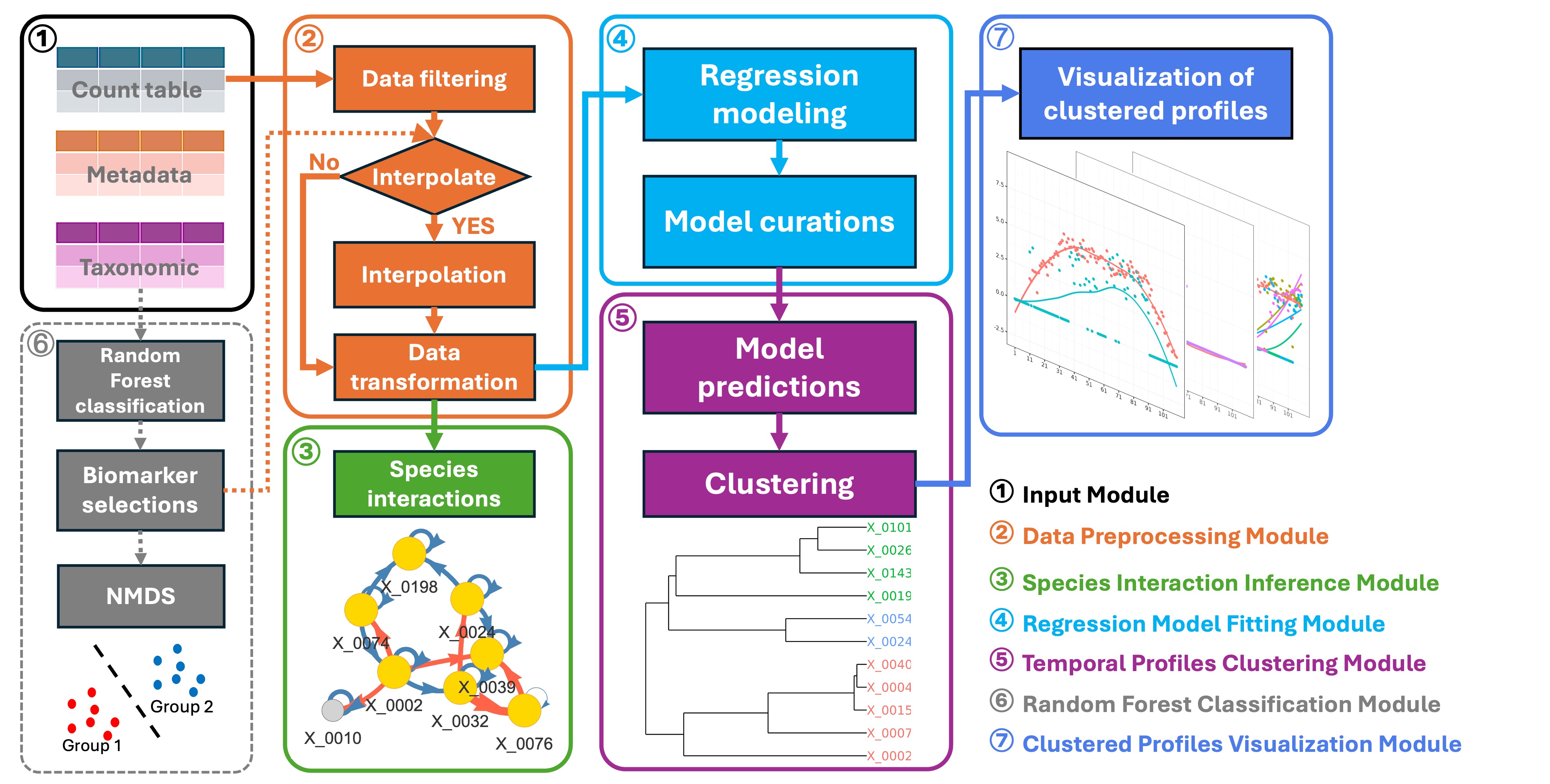
MicrobTiSDA focuses on analyzing microbiome time-series data. Its core functionalities include inferring species interaction relationships within time-series data, constructing abundance time regression models for microbial features, and assessing the similarity of temporal abundance patterns among different microbial features. It integrates the “Learning Interactions from Microbial Time Series” algorithm based on the discrete-time Lotka-Volterra model, and supports the construction of natural spline regression models to characterize changes in microbial feature abundance over time.
You can install the development version of MicrobTiSDA from GitHub with:
# install.packages("devtools")
# library("devtools)
# install_github("Lishijiagg/MicrobTiSDA")Here is an example of applying MicrobTiSDA to an in vitro cultured aquatic microbiome dataset. The dataset was obtained from the study by Fujita et al.
First, we should load MicrobTiSDA and other necessary packages.
library(tidyr)
library(dplyr)
#>
#> Attaching package: 'dplyr'
#> The following objects are masked from 'package:stats':
#>
#>     filter, lag
#> The following objects are masked from 'package:base':
#>
#>     intersect, setdiff, setequal, union
library(ggplot2)
library(MicrobTiSDA)
In this dataset, the in vitro cultivation of aquatic microbiomes was conducted in eight replicate experiments. Each replicate involved continuous cultivation for 110 days, with daily sampling performed throughout the entire period. As a result, a total of 880 aquatic microbiome community samples were obtained. In total, 28 ASVs were detected across all samples.
data("fujita.data")
data("fujita.meta")
data("fujita.taxa")
Please note that MicrobTiSDA has specific format requirements for the user-provided microbiome count table, metadata, and taxonomic annotation files:
head(fujita.data[,c(1:6)])
#>        S_00073 S_00169 S_00265 S_00361 S_00457 S_00553
#> X_0002   11932   10453    8974    4452    6881    6651
#> X_0004       0       0       0       0       0       0
#> X_0007       0       0       0       0       0       0
#> X_0008       0       0       0       0       0       0
#> X_0010       0       0       0       0       0       0
#> X_0015 0 0 0 0 0 0head(fujita.meta[,c(1:6)])
#> time resource inoculum replicate.id treat1 treat2
#> S_00073 1 Medium-C Water Rep.1 Water/Medium-C WC
#> S_00169 2 Medium-C Water Rep.1 Water/Medium-C WC
#> S_00265 3 Medium-C Water Rep.1 Water/Medium-C WC
#> S_00361 4 Medium-C Water Rep.1 Water/Medium-C WC
#> S_00457 5 Medium-C Water Rep.1 Water/Medium-C WC
#> S_00553 6 Medium-C Water Rep.1 Water/Medium-C WChead(fujita.taxa)
#> ID Kingdom Phylum Class
#> X_0001 X_0001 Bacteria Proteobacteria Gammaproteobacteria
#> X_0002 X_0002 Bacteria Proteobacteria Gammaproteobacteria
#> X_0003 X_0003 Bacteria Bacteroidota Bacteroidia
#> X_0004 X_0004 Bacteria Firmicutes Clostridia
#> X_0005 X_0005 Bacteria Proteobacteria Gammaproteobacteria
#> X_0006 X_0006 Bacteria Proteobacteria Gammaproteobacteria
#> Order Family
#> X_0001 Enterobacterales Yersiniaceae
#> X_0002 Aeromonadales Aeromonadaceae
#> X_0003 Chitinophagales Chitinophagaceae
#> X_0004 Peptostreptococcales-Tissierellales Peptostreptococcaceae
#> X_0005 Xanthomonadales Xanthomonadaceae
#> X_0006 Pseudomonadales Pseudomonadaceae
#> Genus Species identified
#> X_0001 Yersinia unidentified Yersinia
#> X_0002 Aeromonas unidentified Aeromonas
#> X_0003 unidentified unidentified Chitinophagaceae
#> X_0004 Clostridioides mangenotii mangenotii
#> X_0005 Stenotrophomonas unidentified Stenotrophomonas
#> X_0006 Pseudomonas unidentified PseudomonasNext, we need to perform filtering on the feature table in this dataset. However, given the relatively small number of microbial features (ASVs) in this dataset, we chose not to filter out ASVs with low abundance or low prevalence.
fujita_filt <- Data.filter(Data = fujita.data,
                          metadata = fujita.meta,
                          OTU_counts_filter_value = 0,
                          OTU_filter_value = 0,
                          Group_var = 'replicate.id')

# The output object of function Data.filter is an S3 class object, use summary() to check the output result.
#summary(fujita_filt)
Typically, the filtered data need to be transformed prior to analysis. MicrobTiSDA provides a modified centered log-ratio (MCLR) transformation for this purpose. This transformation is performed separately for each sampled individual or experimental group; therefore, users are required to specify the grouping variable from the metadata. In this dataset, the variable representing the eight replicate experiments is “replicate.id”.
fujita_trans <- Data.trans(Data = fujita_filt,
                          metadata = fujita.meta,
                          Group_var = 'replicate.id')
After filtering and transforming the dataset, MicrobTiSDA can be used to infer species interactions within each individual subject or replicate microbiome. By integrating the “Learning Interactions from Microbial Time-Series” (LIMITS) framework, MicrobTiSDA is able to infer sparse interaction networks from microbiome time-series data. This step may take a considerable amount of time to complete, depending on the size of the dataset.
fujita_interact <- Spec.interact(Data = fujita_trans,
                                metadata = fujita.meta,
                                Group_var = 'replicate.id',
                                num_iterations = 10)
Next, we can visualize the results of the species interaction inference. The function generates network plots of species interactions for each replicate aquatic microbiome experiment.
fujita_interact_vis <- Interact.dyvis(Interact_data = fujita_interact,
                                     threshold = 1e-6,
                                     core_arrow_num = 4,
                                     Taxa = fujita.taxa)
We can use the function to visualize species interaction networks. The parameter allows users to specify which group or individual to display. For instance, to visualize the species interaction network only for the first replicate experiment (Rep.1) in the dataset, specify . If no group is specified, the network for each group will be plotted by default.
plot(fujita_interact_vis,groups = "Rep.1")
#> Plot: Rep.1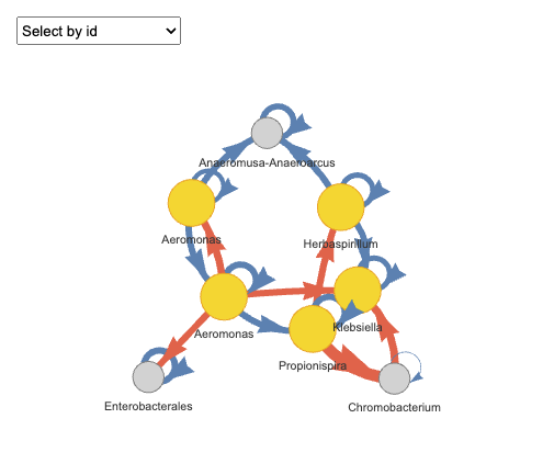
Please note that the output is an interactive HTML chart supporting zooming and dragging for detailed exploration. However, since interactive htmlwidgets cannot be rendered here, users can do it for your own. In the chart, arrow colors indicate interaction types: orange represents positive interactions, and blue represents negative interactions. Nodes represent species, with keystone species (i.e., those involved in multiple pairwise interactions) highlighted in yellow.
After completing species interaction inference for the aquatic microbiome, we can proceed to analyze the temporal abundance patterns of microbial features using MicrobTiSDA. To support this analysis, MicrobTiSDA provides a method for fitting regression models to the abundance trajectories of microbial features. To begin, we first need to construct a design matrix for modeling temporal trends for each microbial feature. This can be accomplished using the function, where users must specify the variables in the metadata that represent the group ID for each subject or replicate, the sample ID, and the time point of each sample.
fujita_design <- Design(metadata = fujita.meta,
                       Group_var = 'replicate.id',
                       Sample_ID = 'timeChar',
                       Pre_processed_Data = fujita_trans,
                       Sample_Time = 'time')
When fitting regression models for each microbial feature, MicrobTiSDA employs natural spline regression. Users can manually specify the positions of spline knots by providing a vector—for example, sets the 10th, 20th, and 30th days in the time series as knot positions. Alternatively, MicrobTiSDA can automatically determine the optimal number and placement of knots using generalized cross-validation, based on a user-defined maximum number of knots .
fujita_model <- Reg.SPLR(Data_for_Reg = fujita_design,
                      pre_processed_data = fujita_trans,
                      max_Knots = 5,
                      unique_values = 5)
here, it is important to account for the sparsity and zero-inflated nature of microbiome data. The function includes the parameter, which specifies the minimum number of non-zero abundance values required across time-series samples for a microbial feature to be included in regression modeling. By default, this threshold is set to at least 5 non-zero values.
Based on the fitted regression models, we can predict the temporal abundance patterns of each microbial feature. These features can then be clustered according to the similarity of their abundance temporal patterns, using correlation distance as the clustering metric.
fujita_model_pred <- Pred.data(Fitted_models = fujita_model,
                              metadata = fujita.meta,
                              Group = 'replicate.id',
                              Sample_Time = 'time',
                              time_step = 1)

fujita_model_clust <- Data.cluster(predicted_data = fujita_model_pred,
                                  clust_method = 'average',
                                  dend_title_size = 12,
                                  font_size = 3)

# Visualize the feature clustering of the first replicate.
plot(fujita_model_clust,groups = "Rep.1")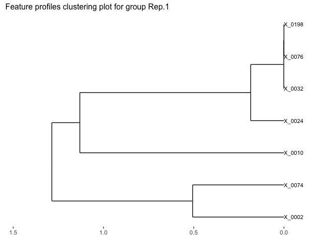
We can also identify the optimal clusters of microbial features based on the clustering results. Here we select features with correlation distance less than 0.15 for clustering.
fujita_clust_results <- Data.cluster.cut(cluster_outputs = fujita_model_clust,
                                        cut_height = 0.15,
                                        font_size = 4)

# Visualize the feature clustering of the first replicate.
plot(fujita_clust_results,groups = "Rep.1")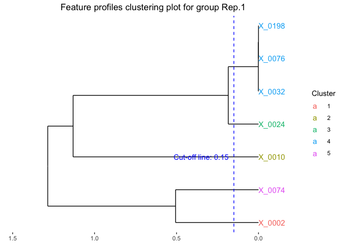
Finally, we can visualize the abundance patterns of microbial features within each selected cluster.
fujita_model_vis <- Data.visual(cluster_results = fujita_clust_results,
cutree_by = 'height',
cluster_height = rep(0.15,8),
predicted_data = fujita_model_pred,
Design_data = fujita_design,
pre_processed_data = fujita_trans,
plot_dots = TRUE,
figure_x_scale = 20,
Taxa = fujita.taxa,
plot_lm = FALSE,
legend_title_size = 10,
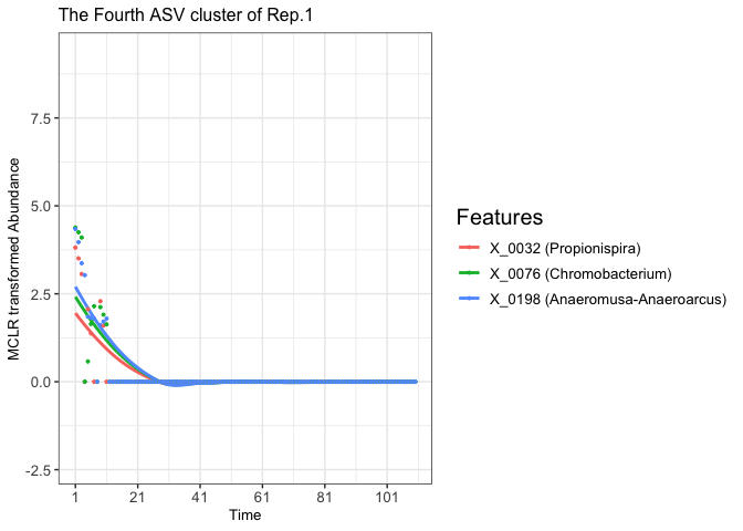
legend_text_size = 10,axis_x_size = 10,axis_title_size = 10,axis_y_size = 10)
# Use plot() to visualize temporal profiles of clustered microbial features.
# For example, we can visualize the fourth feature cluster temporal profiles of the first replicate.
plot(fujita_model_vis, groups = "Rep.1", clusters = 4)
#> In Rep.1, number of feature clusters -- 5
#> `geom_smooth()` using method = 'loess' and formula = 'y ~ x'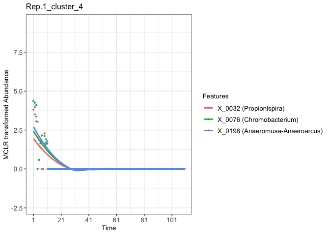
MicrobTiSDA offers users with multiple visualization functions. In addition to the interactive HTML widget for species interaction visualization generated by the function, all other visualization outputs from MicrobTiSDA are structured as ggplot2 objects. Users can extract the underlying ggplot2 object of each visualization and further customize the visual appearance using functions such as and etc. For more information, please refer to .
For example:
# Extract the ggplot2 object of the fourth clustered features from the Rep.1 experimental aquatic microbiome
fujita_vis_rep1_cluster4 <- fujita_model_vis$plots$Rep.1[[4]]
print(fujita_vis_rep1_cluster4)
#> `geom_smooth()` using method = 'loess' and formula = 'y ~ x'
The output objects can be further modified using built-in ggplot2 functions such as and .
# Assume we want to change the title and increase the legend title font size
fujita_vis_rep1_cluster4 <- fujita_vis_rep1_cluster4 +
  theme(legend.title = element_text(size = 15))+
  labs(title = "The Fourth ASV cluster of Rep.1")
print(fujita_vis_rep1_cluster4)
#> `geom_smooth()` using method = 'loess' and formula = 'y ~ x'