![]()
nortsTest is an R package for assessing
normality of stationary processes, it tests if a given data follows a
stationary Gaussian process. The package works as an extension of the
nortest package that performs normality tests in random
samples (independent data). The package’s principal functions
are:
elbouch.test() function that computes the bivariate
El Bouch et
al. test,
epps.test() function that implements the Epps
test,
epps-bootstrap.test() function that implements the
Epps test,
approximating the p-values using a sieve-bootstrap procedure.
lobato.test() function that implements the Lobato
and Velasco’s test,
lobato-bootstrap.test() function that implements the
Lobato and Velasco’s test, approximating the p-values using a
sieve-bootstrap procedure.
rp.test() function that implements the random
projections test of Nieto-Reyes, Cuesta-Albertos and Gamboa’s
test,
vavra.test() function that implements the Psaradakis and Vávra’s
test,
jb-bootstrap.test() function that implements the
Jarque and Bera test, approximating the p-values using a sieve-bootstrap
procedure,
shapiro-bootstrap.test() function that implements
the Shapiro test, approximating the p-values using a sieve-bootstrap
procedure,
cvm-bootstrap.test() function that implements the
Cramer Von Mises test, approximating the p-values using a
sieve-bootstrap procedure.
Additionally, inspired in the function checkresiduals()
of the forecast
package, we provide the check_residuals methods for
checking model’s assumptions using the estimated residuals. The function
checks stationarity, homoscedasticity and normality, presenting a report
of the used tests and conclusions.
library(nortsTest)Classic hypothesis tests for normality such as Shapiro & Wilk,
Anderson & Darling, or Jarque & Bera, do not perform well on
dependent data. Therefore, these tests should not be used to check
whether a given time series has been drawn from a Gaussian process. As a
simple example, we generate a stationary ARMA(1,1) process simulated
using an t student distribution with 7 degrees of freedom, and perform
the Anderson-Darling test from the nortest package.
x = arima.sim(100,model = list(ar = 0.32,ma = 0.25),rand.gen = rt,df = 7)

nortest::ad.test(x)
#>
#>  Anderson-Darling normality test
#>
#> data:  x
#> A = 0.50769, p-value = 0.1954
The null hypothesis is that the data has a normal distribution and therefore, follows a Gaussian Process. At \(\alpha = 0.05\) significance level the alternative hypothesis is rejected and wrongly concludes the data follows a Gaussian process. Applying the Lobato and Velasco’s test of our package, the null hypothesis is correctly rejected.
lobato.test(x)
#>
#>  Lobatos and Velascos test
#>
#> data:  x
#> lobato = 16.864, df = 2, p-value = 0.0002177
#> alternative hypothesis: x does not follow a Gaussian ProcessIn the next example we generate a stationary AR(2) process, using an
exponential distribution with rate of 5, and perform the Epps
and RP with k = 5 random projections tests. With a
significance level at \(\alpha=0.05\),
the null hypothesis of non-normality is rejected.
set.seed(298)
# Simulating the AR(2) process
x = arima.sim(250,model = list(ar =c(0.2,0.3)),rand.gen = rexp,rate = 5)

# tests
epps.test(x)
#>
#>  epps test
#>
#> data:  x
#> epps = 38.158, df = 2, p-value = 5.178e-09
#> alternative hypothesis: x does not follow a Gaussian Process
rp.test(x,k = 5)
#>
#>  k random projections test
#>
#> data:  x
#> k = 5, lobato = 188.771, epps = 28.385, p-value = 0.0007823
#> alternative hypothesis: x does not follow a Gaussian ProcessIn the next example we generate a stationary VAR(1) process of
dimension p = 2, using two independent Gaussian AR(1)
processes, and perform the El Bouch’s test. With a significance
level of \(\alpha = 0.05\), the
alternative hypothesis of non-normality is rejected.
set.seed(298)
# Simulating the VAR(2) process
x1 = arima.sim(250, model = list(ar =c (0.2)))
x2 = arima.sim(250, model = list(ar =c (0.3)))
#
# test
elbouch.test(y = x1, x = x2)
#>
#>  El Bouch, Michel & Comon's test
#>
#> data:  w = (y, x)
#> Z = 0.1438, p-value = 0.4428
#> alternative hypothesis: w = (y, x) does not follow a Gaussian Processcardox dataAs an example, we analyze the monthly mean carbon dioxide (in
ppm) from the astsa package, measured at Mauna Loa
Observatory, Hawaii. from March, 1958 to November 2018. The carbon
dioxide data measured as the mole fraction in dry air, on Mauna Loa
constitute the longest record of direct measurements of CO2 in the
atmosphere. They were started by C. David Keeling of the Scripps
Institution of Oceanography in March of 1958 at a facility of the
National Oceanic and Atmospheric Administration.
library(astsa)
data("cardox")

autoplot(cardox,xlab = "years",ylab = " CO2 (ppm)",color = "darkred",
size = 1,main = "Carbon Dioxide Levels at Mauna Loa")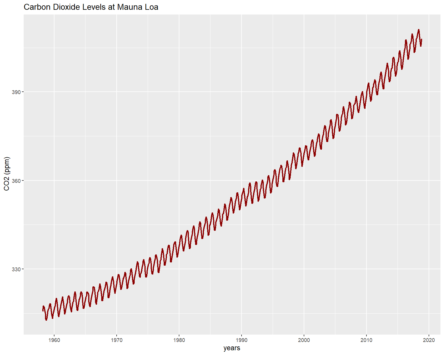
The time series clearly has trend and seasonal components, for analyzing the cardox data we proposed a Gaussian linear state space model. We use the model’s implementation from the forecast package as follows:
library(forecast)
#>
#> Attaching package: 'forecast'
#> The following object is masked from 'package:astsa':
#>
#>     gas

model = ets(cardox)
summary(model)
#> ETS(M,A,A)
#>
#> Call:
#>  ets(y = cardox)
#>
#>   Smoothing parameters:
#>     alpha = 0.5591
#>     beta  = 0.0072
#>     gamma = 0.1061
#>
#>   Initial states:
#>     l = 314.6899
#>     b = 0.0696
#>     s = 0.6611 0.0168 -0.8536 -1.9095 -3.0088 -2.7503
#>            -1.2155 0.6944 2.1365 2.7225 2.3051 1.2012
#>
#>   sigma:  9e-04
#>
#>      AIC     AICc      BIC
#> 3136.280 3137.140 3214.338
#>
#> Training set error measures:
#>                     ME     RMSE       MAE         MPE       MAPE      MASE
#> Training set 0.0232403 0.312003 0.2430829 0.006308831 0.06883992 0.1559102
#>                    ACF1
#> Training set 0.07275949
The best fitted model is a multiplicative level,
additive trend and seasonality state space model. If
the model’s assumptions are satisfied, then the model’s errors behave
like a Gaussian stationary process. These assumptions can be checked
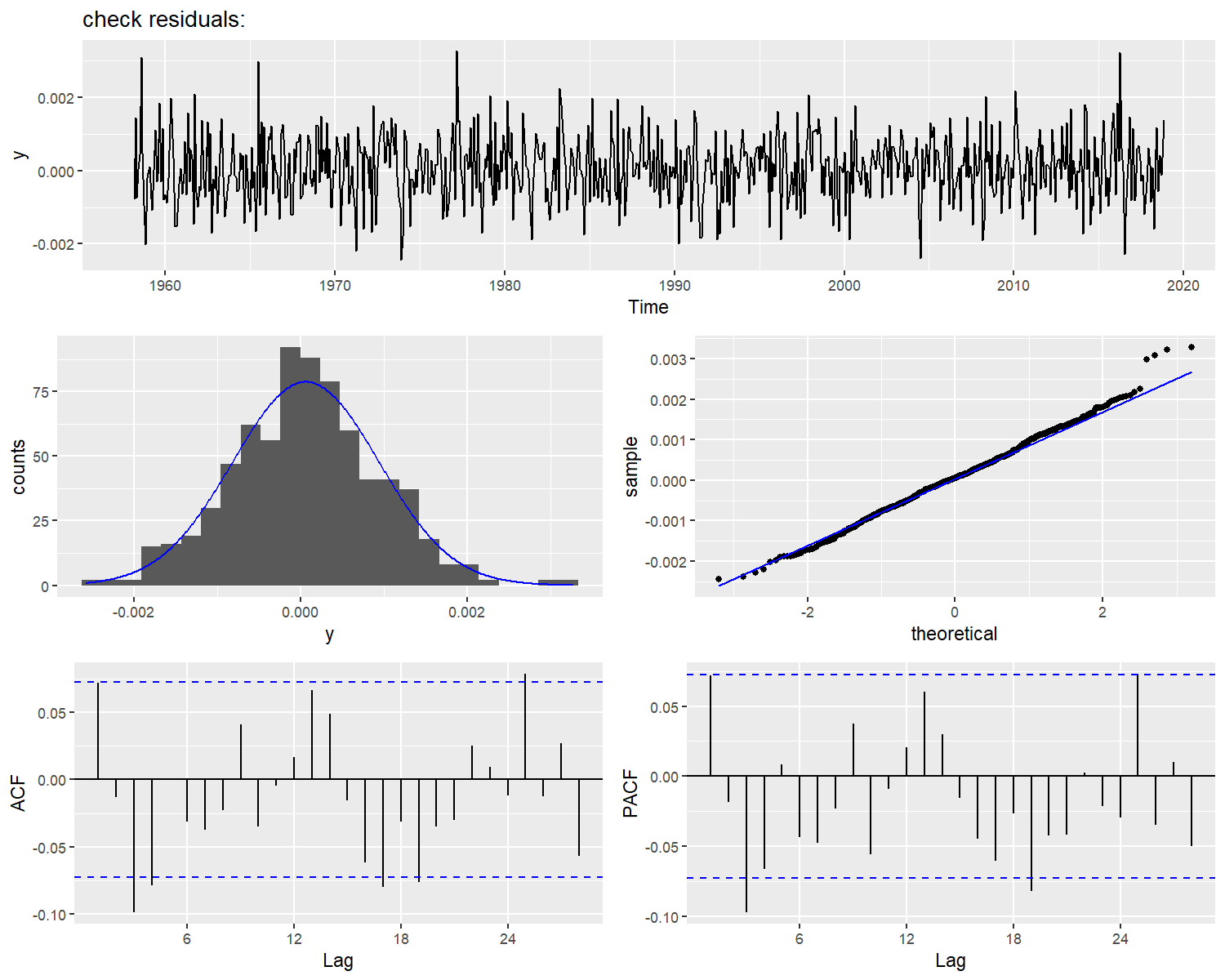
using our check_residuals functions.
In this case, we use an Augmented Dickey-Fuller test for stationary assumption, and a random projections test for normality.
check_residuals(model,unit_root = "adf",normality = "rp",plot = TRUE)
#>
#>  ***************************************************
#>
#>  Unit root test for stationarity:
#>
#>  Augmented Dickey-Fuller Test
#>
#> data:  y
#> Dickey-Fuller = -9.7249, Lag order = 8, p-value = 0.01
#> alternative hypothesis: stationary
#>
#>
#>  Conclusion: y is stationary
#>  ***************************************************
#>
#>  Goodness of fit test for Gaussian Distribution:
#>
#>  k random projections test
#>
#> data:  y
#> k = 2, lobato = 3.8260, epps = 1.3156, p-value = 0.3328
#> alternative hypothesis: y does not follow a Gaussian Process
#>
#>
#>  Conclusion: y follows a Gaussian Process
#>
#>  ***************************************************
After all the model’s assumptions are checked, the model can be used to forecast.
autoplot(forecast(model,h = 12),include = 100,xlab = "years",ylab = " CO2 (ppm)",
         main = "Forecast: Carbon Dioxide Levels at Mauna Loa")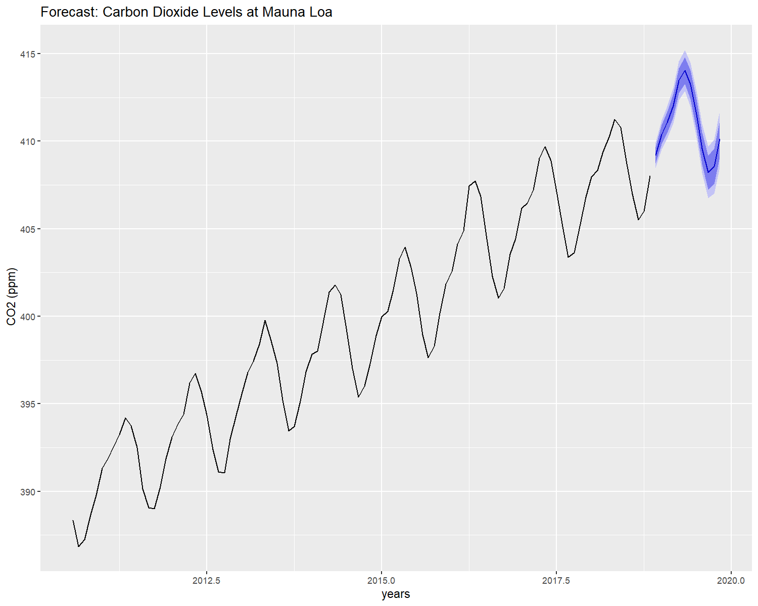
nortsTest?The current development version can be downloaded from GitHub via
if (!requireNamespace("remotes")) install.packages("remotes")

remotes::install_github("asael697/nortsTest",dependencies = TRUE)The nortsTest package offers additional functions for
descriptive analysis in univariate time series.
uroot.test: performs unit root test for checking
stationary in linear time series. The Ljung-Box, Augmented
Dickey-Fuller, Phillips-Perron and Kpps tests can be selected with the
unit_root option parameter.
seasonal.test: performs seasonal unit root test for
stationary in seasonal time series. The hegy,
ch and ocsb tests are available with the
seasonal option parameter.
arch.test: for checking the ARCH effect in time
series. The Ljung-Box and Lagrange Multiplier tests can be selected from
the arch option parameter.
normal.test: for normal distribution check in time
series and random samples. The tests presented above can be chosen for
stationary time series. For random samples (independent data),
the Anderson & Darling, Shapiro & Wilk’s, and Jarque-Bera tests
are available with the normality option parameter.
For visual diagnostic, we offer ggplot2 methods for numeric and time-series data. Most of the functions were adapted from Rob Hyndman’s forecast package.
autoplot: For plotting time series objects
(ts class*).
gghist: histograms for numeric and univariate time
series.
ggnorm: quantile-quantile plot for numeric and
univariate time series.
ggacf & ggpacf: partial and auto
correlation functions plots for numeric and univariate time
series.
check_plot: summary diagnostic plot for univariate
stationary time series.
Currently our check_residuals() and
check_plot() methods are valid for the current models and
classes:
ts: for univariate time series
numeric: for numeric vectors
arima0: from the stats package
Arima: from the forecast
package
fGARCH: from the fGarch
package
lm: from the stats package
glm: from the stats package
Holt and Winters: from the
stats and forecast package
ets: from the forecast package
forecast methods: from the forecast
package.
For overloading more functions, methods or packages, please make a
pull request or send a mail to: asael_am@hotmail.com.
El Bouch, S., Michel, O. & Comon, P. (2022). A normality test for Multivariate dependent samples. Journal of Signal Processing. Volume 201.
Psaradakis, Z. and Vávra, M. (2020) Normality tests for dependent data: large-sample and bootstrap approaches. Communications in Statistics-Simulation and Computation. 49 (2), ISSN 0361-0918.
Psaradakis, Z. & Vávra, M. (2017). A distance test of normality for a wide class of stationary process. Journal of Econometrics and Statistics. 2, 50-60.
Nieto-Reyes, A., Cuesta-Albertos, J. & Gamboa, F. (2014). A random-projection based test of Gaussianity for stationary processes. Computational Statistics & Data Analysis, Elsevier. 75(C), 124-141.
Hyndman, R. & Khandakar, Y. (2008). Automatic time series forecasting: the forecast package for R. Journal of Statistical Software. 26(3), 1-22.
Lobato, I., & Velasco, C. (2004). A simple test of normality for time series. Journal Econometric Theory. 20(4), 671-689.
Epps, T.W. (1987). Testing that a stationary time series is Gaussian. The Annals of Statistic. 15(4), 1683-1698.