Tandem Repeat Analysis from Capillary Electrophoresis (trace)

This package provides a pipeline for short tandem repeat instability analysis from capillary electrophoresis fragment analysis data (e.g fsa files). The main function processes the data and then and then repeat instability metrics are calculated (i.e. expansion index or average repeat gain).

This code is not for clinical use. There are features for accurate repeat sizing if you use validated control samples, but integer repeat units are not returned.

To report bugs or feature requests, please visit the Github issue tracker here. For assistance or any other inquires, contact Zach McLean.

If you use this package, please cite this paper for now.

How to use the package

Either you can use the code described below, or our Shiny app to use an interactive non-coding version.

In this package, each sample is represented by an R6 ‘fragments’ object, which are organized in lists. You usually don’t need to interact with the objects directly. If you do, the attributes of the objects can be accessed with $.

There are several important factors to a successful repeat instability experiment and things to consider when using this package:

(required) Each sample has a unique id, usually the file name
(optional) Baseline control for your experiment. For example, specifying a sample where the modal allele is the inherited repeat length (eg a mouse tail sample) or a sample at the start of a time-course experiment. This is indicated with a TRUE in the metrics_baseline_control column of the metadata. Samples are then grouped together with the metrics_group_id column of the metadata. Multiple samples can be metrics_baseline_control, which can be helpful for the average repeat gain metric to have a more accurate representation of the average repeat at the start of the experiment.
(optional) Batch or repeat length correction for systematic batch effects that occur with repeat-containing amplicons in capillary electrophoresis.
- Repeat containing amplicons do not run linearly with internal ladder sizes in capillary electrophoresis resulting is an underestimation of repeat length if you just convert from base-pair size. These differences are not always consistent across runs which can result in batch effects in the repeat size. So, if the repeat length is to be directly compared for samples from different runs, this batch effect needs to be corrected. This is only relevant when the absolute size of a amplicons are compared for grouping metrics as described above (otherwise instability metrics are all relative and it doesn’t matter that there’s systematic batch effects across runs), when plotting traces from different runs, or if an accurate repeat length is desired.
- There are two main correction approaches that are somewhat related: either ‘batch’ or ‘repeat’ in call_repeats(). Batch correction is relatively simple and just requires you to link samples across batches by indicating them from metadata. But even though the repeat size that is return will be precise, it will not be accurate and underestimates the real repeat length. By contrast, repeat correction can be used to accurately call repeat lengths (which also corrects the batch effects). However, the repeat correction will only be as good as your sample(s) used to call the repeat length, so this can a challenging and advanced feature. You need to use a sample that reliably returns the same peak as the modal peak, or you need to be willing to understand the shape of the distribution and manually validate the repeat length of each control sample for each run.
If starting from fsa files, the GeneScan™ 1200 LIZ™ dye Size Standard ladder assignment may not work very well due to how the ladder assignment algorithm works. It is optimized for scenarios where all peaks of the ladder are resolved, which is usually the case for GeneScan™ 500 LIZ™ or GeneScan™ 600 LIZ™. To work in this package, Ladders like 1200 LIZ™ need to be run on the instrument in such a way that all of the peaks are resolved, otherwise they all blend together at the end. However, these ladders can be fixed by playing with the various parameters (or supplying a truncated version of the GeneScan™ 1200 LIZ™) or manually with the built-in fix_ladders_interactive() app.

Installation

Install the package from CRAN:

install.packages("trace")

Import data

Load the package:

library(trace)

First, we read in the raw data. In this case we will used example data within this package, but usually this would be fsa files that are read in using read_fsa(). The example data is also cloned since the next step modifies the object in place.

fsa_list <- lapply(cell_line_fsa_list, function(x) x$clone())

Alternatively, this is where you would use data exported from Genemapper if you would rather use the Genemapper bp sizing and peak identification algorithms.

fragments_list_genemapper <- genemapper_table_to_fragments(example_data,
  dye_channel = "B",
  min_size_bp = 300
)

Process Samples with `trace`

The trace() function streamlines the processing of fragment analysis data, from ladder assignment to repeat calling. Below is an overview of the key steps that are within trace():

1. Add Metadata

Metadata is used to enable advanced functionality, such as batch correction, repeat correction, and index peak assignment. Prepare a .csv file with the following columns:

Column Name	Purpose	Description
`unique_id`	Required to link up the metadata file with samples	Unique identifier for each sample (e.g., file name). Must be unique across all runs.
`metrics_group_id`	Group samples for instability metrics (e.g., expansion index)	Group ID for samples sharing a common baseline (e.g., mouse ID or experiment group).
`metrics_baseline_control`	Identify baseline samples (e.g., inherited repeat length or day 0)	Set to `TRUE` for baseline control samples (e.g., mouse tail or starting time point).
`batch_run_id`	Group samples by run for batch or repeat correction	Identifier for each fragment analysis run (e.g., date).
`batch_sample_id`	Link samples across runs for batch or repeat correction	Unique ID for each sample across runs.
`batch_sample_modal_repeat`	Specify validated repeat lengths for repeat correction	Validated modal repeat length for samples used in repeat correction.

2. Assign Ladders

Ladder peaks are identified in the ladder channel, and base pair (bp) sizes are predicted for each scan.

Visual Inspection: Always inspect ladders to ensure correct assignment.
Manual Adjustment: If needed, use fix_ladders_interactive() to adjust ladder assignments interactively.

3. Find Fragments

Fragment peaks are identified in the raw trace data. This step transitions the data from a continuous trace to a peak-based representation.

4. Identify Alleles

Identify the main allele (modal peak) for each sample. Can handle samples with two alleles, but metrics are only calculated for the larger of the two.

5. Call Repeats

Base pair sizes are converted to repeat lengths. This step has a lot of additional functionality including:
- Batch correction or accurate repeat sizing.
- Forcing whole repeat units between peaks (usually underestimated in fragment analysis data)

5. Assign Index Peaks

The index peak is the reference repeat length used for instability metrics like expansion index.

Grouped Assignment: Set grouped = TRUE to use the modal peak of baseline control samples (e.g., mouse tail or day 0).
Manual Override: Use index_override_dataframe to manually assign index peaks if needed.

Main function

To carry out this pipeline, call the main function:


fragments_list <- trace(
  fsa_list, 
  min_bp_size = 300,
  grouped = TRUE, 
  metadata_data.frame = metadata,
  show_progress_bar = FALSE)

We can validate that the index peaks were assigned correctly with a dotted vertical line added to the trace. This is perhaps more useful in the context of mice where you can visually see when the inherited repeat length should be in the bimodal distribution.

plot_traces(fragments_list[1], xlim = c(110, 150))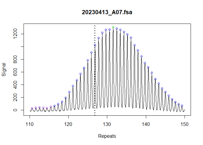

Calculate instability metrics

All of the information we need to calculate the repeat instability metrics has been identified. We can use calculate_instability_metrics() to generate a dataframe of per-sample metrics.

metrics_grouped_df <- calculate_instability_metrics(
  fragments_list = fragments_list,
  peak_threshold = 0.05,
  window_around_index_peak = c(-40, 40)
)

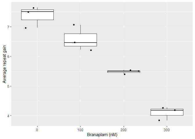
These metrics can then be used to quantify repeat instability. For example, this reproduces a subset of Figure 7e of our manuscript.

library(ggplot2)
library(dplyr)

metrics_grouped_df |>
  left_join(metadata, by = join_by(unique_id)) |>
  filter(
    day > 0,
    modal_peak_signal > 500
  ) |>
  ggplot(aes(as.factor(treatment), average_repeat_change)) +
    geom_boxplot() +
    geom_jitter() +
    labs(y = "Average repeat gain",
         x = "Branaplam (nM)")